Joints
Joint Basics
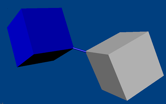
A joint constrains the way two actors move relative to one another. A typical use for a joint would be to model a door hinge or the shoulder of a character. A variety of joint types are implemented in the PhysX extensions library. Custom joints may also be implemented.
The creation of simple joints and limits is demonstrated in the SnippetJoint snippet.
To create a joint, call the joint’s creation function PxRevoluteJointCreate():
PxRevoluteJointCreate(PxPhysics& physics,
                      PxRigidActor* actor0, const PxTransform& localFrame0,
                      PxRigidActor* actor1, const PxTransform& localFrame1);
This has the same pattern for all joints: two actors, and for each actor a constraint frame.
One of the actors must be movable, either a PxRigidDynamic or a PxArticulationLink. The other may be of one of those types, or a PxRigidStatic. Use a NULL pointer here to indicate an implicit actor representing the immovable global reference frame.
Each localFrame argument specifies a constraint frame relative to the actor’s global pose. Each joint defines a relationship between the global positions and origins of the constraint frames that will be enforced by the PhysX constraint solver. In this example, the revolute joint constrains the origin points of the two frames to be coincident and their x-axes to coincide, but allows the two actors to rotate freely relative to one another around this common axis.
PhysX supports the following joint types:
a
PxFixedJointlocks the orientations and origins rigidly togethera
PxDistanceJointkeeps the origins within a certain distance rangea
PxSphericalJoint(also called a ball-and-socket) keeps the origins together, but allows the orientations to vary freely.a
PxRevoluteJoint(also called a hinge) keeps the origins and x-axes of the frames together, and allows free rotation around this common axis.a
PxPrismaticJoint(also called a slider) keeps the orientations identical, but allows the origin of each frame to slide freely along the common x-axis.a
PxGearJointuses a gear ratio to couple the rotations of two revolute joints.a
PxRackAndPinionJointuses a gear ratio (rotation/distance) to couple the rotation of a revolute joint to the travel of a prismatic joint.a
PxD6Jointjoint is a highly configurable joint that allows specification of individual degrees of freedom either to move freely or be locked together. It can be used to implement a wide variety of mechanical and anatomical joints, but is somewhat less intuitive to configure than the other joint types. This joint is covered in detail below.
All joints are implemented as plugins to the SDK through the PxConstraint class. A number of the properties for each joint are configured using the PxConstraintFlag enumeration.
Note
As in the rest of the PhysX API, all joint angles for limits and drive targets are specified in radians.
Visualization
All standard PhysX joints support debug visualization. You can visualize the joint frames of each actor, and also any limits the joint may have.
By default, joints are not visualized. To visualize a joint, set its visualization constraint flag and the appropriate scene-level visualization parameters:
scene->setVisualizationParameter(PxVisualizationParameter::eJOINT_LOCAL_FRAMES, 1.0f);
scene->setVisualizationParameter(PxVisualizationParameter::eJOINT_LIMITS, 1.0f);

...

joint->setConstraintFlag(PxConstraintFlag::eVISUALIZATION)
Force Reporting
The force applied at a joint may be retrieved after simulation with a call to getForce():
scene->fetchResults(...);
joint->getConstraint().getForce(force, torque);
The force is specified in the world frame.
Note that this force is only updated while the joint’s actors are awake.
Breakage
All of the standard PhysX joints can be made breakable. A maximum breaking force and torque may be specified. If the force or torque required to maintain the joint constraint exceeds either threshold, the joint will break. Breaking a joint generates a simulation event (see onConstraintBreak()), and the joint no longer participates in simulation, although it remains attached to its actors until it is deleted.
By default the threshold force and torque are set to PX_MAX_REAL, making joints effectively unbreakable. To make a joint breakable, specify the force and torque thresholds:
const PxReal forceThreshold = 100.0f;
const PxReal torqueThreshold = 200.0f;
joint->setBreakForce(forceThreshold, torqueThreshold);
A constraint flag records whether a joint is currently broken:
bool broken = (joint->getConstraintFlags() & PxConstraintFlag::eBROKEN) != 0;
Breaking a joint causes a callback via onConstraintBreak(). In this callback, a pointer to the joint and its type are specified in the PxConstraintInfo::externalReference and PxConstraintInfo::type fields of the PxConstraintInfo struct. For custom joint types it is recommended to use the PxConstraintInfo::type field to determine the dynamic type of the broken constraint. Otherwise, simply cast the externalReference to a PxJoint:
class MySimulationEventCallback
{
    void onConstraintBreak(PxConstraintInfo* constraints, PxU32 count)
    {
        for(PxU32 i=0; i<count; i++)
        {
            if(PxConstraintExtIDs::eJOINT == constraints[i].type)
            {
                PxJoint* joint = reinterpret_cast<PxJoint*>(constraints[i].externalReference);
                ...
            }
            else
            if(eUSER_CUSTOM_JOINT == constraints[i].type)
            {
                CustomUserType* customUserType = reinterpret_cast<CustomUserType*>(constraints[i].externalReference);
                ...
            }
        }
    }
}
Limits
Some PhysX joints constrain not just relative rotation or translation, but can also enforce limits on the range of that motion. For example, in its initial configuration the revolute joint allows free rotation around its axis. This free rotation can be limited to to a range of angles by specifying a lower and upper limit and configuring the joint as a limited joint. The class PxRevoluteJoint serves as a good example:
revolute->setLimit(PxJointAngularLimitPair(-PxPi/4, PxPi/4));
revolute->setRevoluteJointFlag(PxRevoluteJointFlag::eLIMIT_ENABLED, true);
Limits may be either hard or soft. When a hard limit is reached, relative motion will simply stop dead if the limit is configured with zero restitution, or bounce if the restitution is non-zero. When a soft limit is violated, the solver will pull the joint back towards the limit using a spring specified by the limit’s spring and damping parameters. By default, limits are hard and without restitution, so when the joint reaches a limit motion will simply stop. To specify softness for a limit, declare the limit structure and set the spring and damping parameters directly:
PxJointAngularLimitPair limitPair(-PxPi/4, PxPi/4);
limitPair.spring = 100.0f;
limitPair.damping = 20.0f;
revolute->setRevoluteJointLimit(limitPair);
revolute->setRevoluteJointFlag(PxRevoluteJointFlag::eLIMIT_ENABLED, true);
Actuation
Some PhysX joints may be actuated by a motor or a spring implicitly integrated by the PhysX solver. While driving simulations with actuated joints is more expensive than simply applying forces, it can provide much more stable control of simulation. See D6 Joint, Prismatic Joint, and Revolute Joint for details.
Note
The force generated by actuation is not included in the force reported by the solver, nor does it contribute towards exceeding the joint’s breakage force threshold.
Note
Changing the drive parameters for a joint, or activating or deactivating the drive, does not wake sleeping bodies attached to the joint. If required, wake these bodies manually.
When using spring drives (in particular, drives on the D6 joint), the flag PxD6JointDriveFlag::eACCELERATION is strongly recommended. This flag will automatically scale the strength of the spring according to the masses and inertias of objects that the limit is acting upon, and can substantially reduce the amount of tuning required for good, stable behavior.
Mass Scaling
PhysX joints may apply scale to the mass and moment of inertia of the two connected bodies for the purposes of resolving a joint. For example, if two objects in a ragdoll have masses 1 and 10, PhysX will typically resolve the joint by changing the velocity of the lighter body much more than the heavier one. A mass scale of 10 may be applied to the first body to make PhysX change the velocity of both bodies by an equal amount. To ensure the same property holds for both linear and angular velocity, the inertia scales may also be adjusted in accordance with the bodies’ inertias. Applying mass scales such that the joint sees similar effective masses and inertias makes the solver converge faster, which can make individual joints seem less rubbery or separated, and sets of jointed bodies appear less twitchy.
Many applications that prioritize visual behavior over adherence to physical laws can benefit from tuning these scale values. It is worth noting that mass and inertia scaling is fundamentally nonphysical. In general momentum will not be conserved, the energy of the system may increase, the force reported for the joint may be incorrect, and non-physical tuning of breakage thresholds and force limits may be required.
Fixed Joint
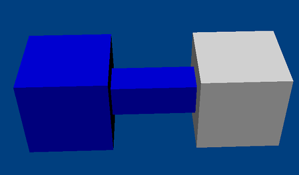
The fixed joint PxFixedJoint constrains two objects so that the positions and orientations of their constraint frames are the same.
Note
All joints are enforced by the dynamics solver, so although under ideal conditions the objects will maintain their spatial relationship, there may be some drift. A common alternative, which is cheaper to simulate and does not suffer from drift, is to construct a single actor with multiple shapes. However fixed joints are useful, for example, when a joint must be breakable or report its constraint force.
Spherical Joint
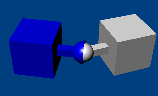
A spherical joint PxSphericalJoint constrains the origins of the actor’s constraint frames to be coincident.
The spherical joint supports a cone limit, which constrains the angle between the X-axes of the two constraint frames. Actor1’s X-axis is constrained by a limit cone whose axis is the x-axis of actor0’s constraint frame. The allowed limit values are the maximum rotation around the y- and z- axes of that frame. Different values for the y- and z- axes may be specified, in which case the limit takes the form of an elliptical angular cone:
joint->setLimitCone(PxJointLimitCone(PxPi/2, PxPi/6, 0.01f);
joint->setSphericalJointFlag(PxSphericalJointFlag::eLIMIT_ENABLED, true);
Note that very small or highly elliptical limit cones may result in solver jitter.
Note
Visualization of the limit surface can help considerably in understanding its shape.
Revolute Joint
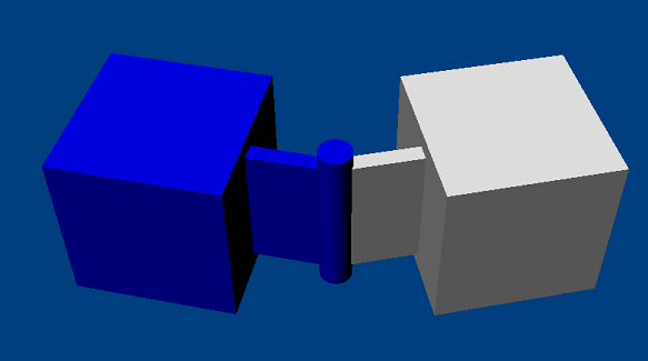
A revolute joint PxRevoluteJoint removes all but a single rotational degree of freedom from two objects. The axis along which the two bodies may rotate is specified by the common origin of the joint frames and their common x-axis. In theory, all origin points along the axis of rotation are equivalent, but simulation stability is best in practice when the point is near where the bodies are closest.
The joint supports a rotational limit with upper and lower extents. The angle is zero where the y- and z- axes of the joint frames are coincident, and increases moving from the y-axis towards the z-axis:
joint->setLimit(PxJointAngularLimitPair(-PxPi/4, PxPi/4, 0.01f);
joint->setRevoluteJointFlag(PxRevoluteJointFlag::eLIMIT_ENABLED, true);
The joint also supports a motor which drives the relative angular velocity of the two actors towards a user-specified target velocity. The magnitude of the force applied by the motor may be limited to a specified maximum:
joint->setDriveVelocity(10.0f);
joint->setRevoluteJointFlag(PxRevoluteJointFlag::eDRIVE_ENABLED, true);
By default, when the angular velocity at the joint exceeds the target velocity the motor acts as a brake; a freespin flag PxRevoluteJointFlag::eDRIVE_FREESPIN disables this braking behavior.
The drive force limit for a revolute joint may be interpreted either as a force or an impulse, depending on the value of PxConstraintFlag::eDRIVE_LIMITS_ARE_FORCES.
Prismatic Joint
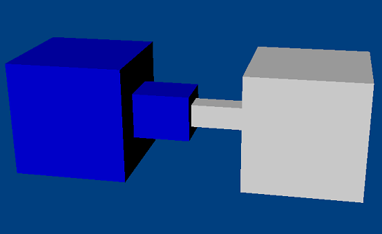
A prismatic joint PxPrismaticJoint prevents all rotational motion, but allows the origin of actor1’s constraint frame to move freely along the x-axis of actor0’s constraint frame. The prismatic joint supports a single limit with upper and lower bounds on the distance between the two constraint frames’ origin points:
joint->setLimit(PxJointLinearLimitPair(-10.0f, 20.0f, 0.01f);
joint->setPrismaticJointFlag(PxPrismaticJointFlag::eLIMIT_ENABLED, true);
Distance Joint
The distance joint PxDistanceJoint keeps the origins of the constraint frames within a certain range of distance. The range may have both upper and lower bounds, which are enabled separately by flags:
joint->setMaxDistance(10.0f);
joint->setDistanceJointFlag(eMAX_DISTANCE_ENABLED, true);
Motion beyond the maximum distance may either be entirely prevented by the solver, or pushed back towards its range with an implicit spring, for which spring and damping parameters may be specified.
Gear Joint
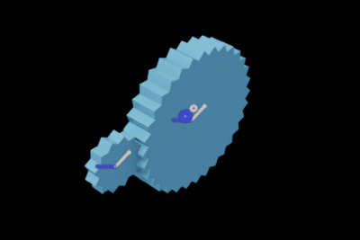
The gear joint PxGearJoint uses a gear ratio to constrain the relative angular velocity of the two bodies of the joint. Additionally, it contrains the relative position of the two bodies of the joint.
It is required that the two bodies of the gear joint rotate only around the twist axis. The requirement for each body may in turn be enforced by additional joints such as PxRevoluteJoint or PxD6Joint configured with a single rotational degree of freedom around PxD6Axis::eTWIST. PxGearJoint also allows either or both of the bodies to be of type PxArticulationLink. This being the case, the inbound PxArticulationJointReducedCoordinate should be configured to be of type PxArticulationJointType::eREVOLUTE or PxArticulationJointType::eREVOLUTE_UNWRAPPED:
gearJoint->setJoints(hinge0, hinge1);
rackJoint->setGearRatio(gearRatio);
Rack And Pinion Joint
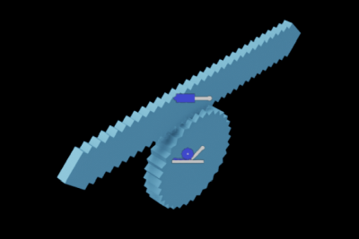
The gear joint PxGearJoint uses a gear ratio to enforce a relationship between the angular velocity of one body and the linear velocity of another. Additionally, it contrains the relative position of the two bodies of the joint.
It is required that one body of the pair has a single translational degree of freedom. A further requirement is that the other body of the pair has a single rotational degree of freedom. These requirements may be enforced in turn by additional joints. For example, the requirement of translational motion may be enforced with PxPrismaticJoint or PxD6Joint configured with a single translational degree of freedom along PxD6Axis::eX. Likewise, the requirement of rotational motion may be enforced with PxRevoluteJoint or a PxD6Joint configured with a single rotational degree of freedom around PxD6Axis::eTWIST. Either or both of the bodies may be of type PxArticulationLink. This being the case, the inbound PxArticulationJointReducedCoordinate should be configured to be PxArticulationJointType::eREVOLUTE or PxArticulationJointType::eREVOLUTE_UNWRAPPED for the rotating body and PxArticulationJointType::ePRISMATIC for the translating body:
rackAndPinionJoint->setJoints(hinge0, prismatic);
rackAndPinionJoint->setData(nbRackTeeth, nbPinionTeeth, rackLength);
D6 Joint
The D6 joint PxD6Joint is by far the most complex of the standard PhysX joints. In its default state it behaves like a fixed joint - that is, it rigidly fixes the constraint frames of its two actors. However, individual degrees of freedom may be unlocked to permit any combination of rotation around the x-, y- and z- axes, and translation along these axes.
Locking and Unlocking Axes
To unlock and lock degrees of freedom, use the PxD6Joint::setMotion() function:
d6joint->setMotion(PxD6Axis::eX, PxD6Motion::eFREE);
Unlocking translational degrees of freedom allows the origin point of actor1’s constraint frame to move along a subset of the axes defined by actor0’s constraint frame. For example, unlocking just the X-axis creates the equivalent of a prismatic joint.
Rotational degrees of freedom are partitioned as twist (around the X-axis of actor0’s constraint frame) and swing (around the Y- and Z- axes). Different effects are achieved by unlocking various combinations of twist and swing.
if just a single degree of angular freedom is unlocked, the result is always equivalent to a revolute joint. It is recommended that if just one angular freedom is unlocked, it should be the twist degree, because the joint has various configuration options and optimizations that are designed for this case.
if both swing degrees of freedom are unlocked but the twist degree remains locked, the result is a zero-twist joint. The x-axis of actor1 swings freely away from the x-axis of actor0 but twists to minimize the rotation required to align the two frames. This creates a kind of isotropic universal joint which avoids the problems of the usual ‘engineering style’ universal joint (see below) that is sometimes used as a kind of twist constraint. There is a nasty singularity at π radians (180 degrees) swing, so a swing limit should be used to avoid the singularity.
if one swing and one twist degree of freedom are unlocked but the remaining swing is kept locked, a zero-swing joint results (often also called a universal joint). If for example the SWING1 (y-axis rotation) is unlocked, the x-axis of actor1 is constrained to remain orthogonal to the z-axis of actor0. In character applications, this joint can be used to model an elbow swing joint incorporating the twist freedom of the lower arm or a knee swing joint incorporating the twist freedom of the lower leg. In vehicle applications, these joints can be used as ‘steered wheel’ joints in which the child actor is the wheel, free to rotate about its twist axis, while the free swing axis in the parent acts as the steering axis. Care must be taken with this combination because of anisotropic behavior and singularities (beware the dreaded gimbal lock) at angles of π/2 radians (90 degrees), making the zero-twist joint a better behaved alternative for most use cases.
if all three angular degrees are unlocked, the result is equivalent to a spherical joint.
Common use cases can be implemented as follows:
The cylindrical joint (with axis along the common x-axis of the two constraint frames) is given by the combination:
d6joint->setMotion(PxD6Axis::eX,     PxD6Motion::eFREE);
d6joint->setMotion(PxD6Axis::eTWIST, PxD6Motion::eFREE);
the point-on-plane joint (with plane axis along the x-axis of actor0’s constraint frame) is given by the combination:
d6joint->setMotion(PxD6Axis::eY,      PxD6Motion::eFREE);
d6joint->setMotion(PxD6Axis::eZ,      PxD6Motion::eFREE);
d6joint->setMotion(PxD6Axis::eTWIST,  PxD6Motion::eFREE);
d6joint->setMotion(PxD6Axis::eSWING1, PxD6Motion::eFREE);
d6joint->setMotion(PxD6Axis::eSWING2, PxD6Motion::eFREE);
the point-on-line joint (with axis along the x-axis of actor0’s constraint frame) is given by the combination:
d6joint->setMotion(PxD6Axis::eX,      PxD6Motion::eFREE);
d6joint->setMotion(PxD6Axis::eTWIST,  PxD6Motion::eFREE);
d6joint->setMotion(PxD6Axis::eSWING1, PxD6Motion::eFREE);
d6joint->setMotion(PxD6Axis::eSWING2, PxD6Motion::eFREE);
Limits
Any axis configured as free may also be specified as limited. The D6 supports different limits which may be used in any combination.
A single linear limit with only an upper bound is used to constrain any of the translational degrees of freedom. The limit constrains the distance between the origins of the constraint frames when projected onto these axes. For example, the combination:
d6joint->setMotion(PxD6Axis::eX, PxD6Motion::eFREE);
d6joint->setMotion(PxD6Axis::eY, PxD6Motion::eLIMITED);
d6joint->setMotion(PxD6Axis::eZ, PxD6Motion::eLIMITED);
d6joint->setDistanceLimit(PxJointLinearLimit(1.0f, 0.1f));
constrains the y- and z- coordinates of actor1’s constraint frame to lie within the unit disc. Since the x-axis is unconstrained, the effect is to constrain the origin of actor1’s constraint frame to lie within a cylinder of radius 1 extending along the x-axis of actor0’s constraint frame.
The D6 joint also supports per-axis linear limit pairs, with the setLinearLimit() function. This can be used to implement a prismatic joint when only one of the linear axis is limited and the others remain locked. Otherwise in 2D and 3D this gives birth to quad-shaped and box-shaped limit volumes, as opposed to the disc-shaped and sphere-shaped volumes generated by PxD6Joint::setDistanceLimit.
The twist degree of freedom is limited by a pair limit with upper and lower bounds, identical to the limit of the revolute joint.
If both swing degrees of freedom are limited, a limit cone is generated, identical to the limit of the spherical joint. As with the spherical joint, very small or highly elliptical limit cones may result in solver jitter.
If only one swing degree of freedom is limited, the corresponding angle from the cone limit is used to limit rotation. If the other swing degree is locked, the maximum value of the limit is π radians (180 degrees). If the other swing degree is free, the maximum value of the limit is π/2 radians (90 degrees).
Drives
The D6 has a linear drive model, and two possible angular drive models. The drive is a proportional derivative drive, which applies a force as follows:
force = spring * (targetPosition - position) + damping * (targetVelocity - velocity)
The drive model may also be configured to generate a proportional acceleration instead of a force, factoring in the masses of the actors to which the joint is attached. Acceleration drive is often easier to tune than force drive.
- The linear drive model for the D6 has the following parameters:
target position, specified in actor0’s constraint frame
target velocity, specified in actor0’s constraint frame
spring
damping
forceLimit - the maximum force the drive can apply
acceleration drive flag
The drive attempts to follow the desired position input with the configured stiffness and damping properties. A physical lag due to the inertia of the driven body acting through the drive spring will occur; therefore, sudden step changes will result over a number of time steps. Physical lag can be reduced by stiffening the spring or supplying a velocity target.
With a fixed position input and a zero target velocity, a position drive will spring about that drive position with the specified springing/damping characteristics:
// set all translational degrees free

d6joint->setMotion(PxD6Axis::eX, PxD6Motion::eFREE);
d6joint->setMotion(PxD6Axis::eY, PxD6Motion::eFREE);
d6joint->setMotion(PxD6Axis::eZ, PxD6Motion::eFREE);

// set all translation degrees driven:

PxD6Drive drive(10.0f, -20.0f, PX_MAX_F32, true);
d6joint->setDrive(PxD6JointDrive::eX, drive);
d6joint->setDrive(PxD6JointDrive::eY, drive);
d6joint->setDrive(PxD6JointDrive::eZ, drive);

// Drive the joint to the local(actor[0]) origin - since no angular
// dofs are free, the angular part of the transform is ignored

d6joint->setDrivePosition(PxTransform(1.0f));
d6joint->setDriveVelocity(PxVec3(PxZero));
Angular drive differs from linear drive in a fundamental way: it does not have a simple and intuitive representation free from singularities. For this reason, the D6 joint provides two angular drive models - twist and swing and SLERP (Spherical Linear Interpolation).
The two models differ in the way they estimate the path in quaternion space between the current orientation and the target orientation. In a SLERP drive, the quaternion is used directly. In a twist and swing drive, it is decomposed into separate twist and swing components and each component is interpolated separately. Twist and swing is intuitive in many situations; however, there is a singularity when driven to 180 degrees swing. In addition, the drive will not follow the shortest arc between two orientations. On the other hand, SLERP drive will follow the shortest arc between a pair of angular configurations, but may cause unintuitive changes in the joint’s twist and swing.
The angular drive model has the following parameters:
An angular velocity target specified relative to actor0’s constraint frame
An orientation target specified relative to actor0’s constraint frame
drive specifications for SLERP (slerpDrive), swing (swingDrive) and twist (twistDrive):
spring - amount of torque needed to move the joint to its target orientation proportional to the angle from the target (not used for a velocity drive).
damping - applied to the drive spring (used to smooth out oscillations about the drive target).
forceLimit - the maximum torque the drive can apply.
acceleration drive flag. If this flag is set the acceleration (rather than the force) applied by the drive is proportional to the angle from the target.
Best results will be achieved when the drive target inputs are consistent with the joint freedom and limit constraints.
Note
if any angular degrees of freedom are locked, the SLERP drive parameters are ignored. If all angular degrees of freedom are unlocked, and parameters are set for multiple angular drives, the SLERP parameters will be used.
Configuring PhysX Joint Types for Best Behavior
The behavior quality of joints in PhysX is largely determined by the ability of the iterative solver to converge. Better convergence can be achieved simply by increasing the attributes of the PxRigidDynamic which controls the solver iteration count. However, joints can also be configured to produce better convergence.
the solver can have difficulty converging well when a light object is constrained between two heavy objects. Mass ratios of higher than 10 are best avoided in such scenarios.
when one body is significantly heavier than the other, make the lighter body the second actor in the joint. Similarly, when one of the objects is static or kinematic (or the actor pointer is NULL) make the dynamic body the second actor.
A common use for joints is to move objects around in the world. Best results are obtained when the solver has access to the velocity of motion as well as the change in position.
if very stiff controller is desired that moves the object to specific position each frame, consider jointing the object to a kinematic actor and use the setKinematicTarget function to move the actor.
if a more springy controller is desired, use a D6 joint with a drive target to set the desired position and orientation, and control the spring parameters to increase stiffness and damping. In general, acceleration drive is much easier to tune than force drive.
Custom Constraints
It is also possible to add new joint types to PhysX. Use the existing joints in the PhysXExtensions library as a reference, and also the source for SnippetCustomJoint, which shows how to implement a Pulley Joint. Serializing custom objects is discussed in the chapter Serialization, so the discussion here is limited to how to achieve the desired behavior in simulation. This is an advanced topic, and assumes familiarity with the mathematics underlying rigid body simulation. The presentation here assumes that the joint constrains two bodies; the case for a static body is equivalent to a dynamic body of infinite mass.
The functions which implement dynamic behavior of joints are PhysX shaders, similar in nature to the PxFilterShader (see Collision Filtering). In particular, the functions may execute in parallel and asynchronously, and should not access any state except that passed in as parameters.
To create a custom joint class, define the following:
the functions which implement the behavior of the constraint. The functions must be stateless, because they may be called simultaneously from multiple threads. When each function is called, PhysX passes a constant block which can be used to store the joint configuration parameters (offsets, axes, limits etc).
a static instance of PxConstraintShaderTable containing pointers to the functions
a class implementing the PxConstraintConnector interface, that connects the custom joint to PhysX.
Defining Constraint Behavior
The most important function that defines the joint behavior is the solver preparation function, which generates inputs to PhysX’ velocity-based constraint solver.
The processing sequence during simulation is as follows:
in the simulate() function, before starting simulation the scene updates an internal copy of the joint’s constant block (so that the joint’s copy may be modified during simulation without causing races).
collision detection runs, and may wake bodies. If the joint connects two bodies, the simulation will ensure that either both bodies are awake, or neither is.
for every joint connected to an awake body, the simulation calls the solver preparation function.
the solver updates body velocities and positions.
The Solver Preparation Function
The solver preparation function for a joint has the following signature:
PxU32 prepare(Px1DConstraint* constraints,
              PxVec3& bodyAWorldOffset,
              PxU32 maxConstraints,
              PxConstraintInvMassScale &invMassScale,
              const void* constantBlock,
              const PxTransform& bodyAToWorld,
              const PxTransform& bodyBToWorld,
              bool useExtendedLimits,
              PxVec3p& cAtW,
              PxVec3p& cBtW);
The parameters are as follows:
constraints is the output buffer of constraint rows.
bodyAWorldOffset is the point, specified in world space as an offset from the origin of bodyA, at which the constraint forces act to enforce the joint. The constraint solver ignores this value as the information is already encoded in the constraint array, but when reporting forces it is necessary to choose a point at which the force is considered to act. For PhysX joints, the attachment point of the joint on body B is used.
maxConstraints is the size of the buffer, which limits the number of constraint rows that may be generated.
invMassScale is the inverse mass scales which should be applied to the bodies for the purpose of resolving the joint. In the standard joints, these are just the joint’s mass scaling parameters (see Mass Scaling).
constantBlock is the simulation’s copy of the joint constant block.
bodyAToWorld is the center of mass frame of the first constrained body (the identity transform if the first actor is static, or if a NULL actor pointer was provided for it).
bodyBToWorld is the center of mass frame of the second constrained body (the identity transform if the second actor is static, or if a NULL actor pointer was provided for it)
useExtendedLimits enables angular limit ranges outside of (-PI, PI).
cAtW is the world space location of body A’s joint frame (position only).
cBtW is the world space location of body B’s joint frame (position only)
The role of the solver preparation function is to populate the buffer of Px1DConstraints, provide the point of application for force reporting, and provide the mass scaling properties. The return value is the number of Px1DConstraints generated in the output buffer.
Notice that although the joint parameters (relative pose etc) are typically specified relative to an actor, the solver preparation function works with the transforms of the underlying rigid bodies. The constraint infrastructure (see Data Management) assists joints in maintaining consistency when, for example, the application modifies the center of mass of an actor.
Each Px1DConstraint constrains one degree of freedom between the two bodies. The structure looks like this:
struct Px1DConstraint
{
    PxVec3                linear0;
    PxReal                geometricError;
    PxVec3                angular0;
    PxReal                velocityTarget;

    PxVec3                linear1;
    PxReal                minImpulse;
    PxVec3                angular1;
    PxReal                maxImpulse;

    union
    {
        struct SpringModifiers
        {
            PxReal        stiffness;
            PxReal        damping;
        } spring;
        struct RestitutionModifiers
        {
            PxReal        restitution;
            PxReal        velocityThreshold;
        } bounce;
    } mods;

    PxReal               forInternalUse;
    PxU16                flags;
    PxU16                solveHint;
}
Each Px1DConstraint is either a hard constraint (for example, one axis of a fixed joint) or a soft constraint (for example, a spring). A joint may have a mixture of hard and soft constraint rows - for example, the actuated joint at a rag doll shoulder often has:
3 hard 1D-constraints which prevent the shoulder from separating.
3 hard 1D-constraints constraining the angular degrees of freedom within some limits.
3 soft constraints simulating resistance to angular motion from muscles.
The constraint is treated as hard unless the Px1DConstraintFlag::eSPRING flag is set.
For both soft and hard constraints, the solver velocity for each row is the quantity:
v = body0vel.dot(lin0, ang0) - body1vel.dot(lin1, ang1)
Hard Constraints
For a hard constraint, the solver attempts to generate:
a set of motion solver velocities vMotion for objects which, when integrated, respect the constraint errors, represented by the equation:
vMotion + (geometricError / timestep) = velocityTarget
a set of post-simulation solver velocities vNext for the objects which respect the constraints:
vNext = velocityTarget
The motion velocities are used for integration and then discarded. The post-simulation velocities are the values that getLinearVelocity() and getAngularVelocity() return.
There are two special options for hard constraints, both most often used to implement limits: restitution and velocity biasing. They are set by the constraint flags Px1DConstraintFlag::eRESTITUTION and Px1DConstraintFlag::eKEEPBIAS, are mutually exclusive, and restitution takes priority (in the sense that if restitution is set, biasing is ignored).
Restitution simulates bouncing (off a limit, for example). If the impact solver velocity vCurrent at the start of simulation exceeds the restitution velocity threshold, the target velocity of the constraint will be set to:
restitution * -vCurrent
and the input velocityTarget field will be ignored. To use restitution, set Px1DConstraintFlag::eRESTITUTION.
Velocity biasing generates post-simulation velocities to satisfy the same constraints as for the motion velocities:
vNext + (geometricError / timestep) = velocityTarget
This can be useful if, for example, the joint is approaching a limit but has not yet reached it. If the target velocity is 0 and the geometric error is the distance remaining to the limit, the solver will constrain the velocity below that required to violate the limit after integration. The joint should then converge smoothly to the limit.
Soft Constraints
Alternatively, the solver can attempt to resolve the velocity constraint as an implicit spring. In this case, the motion velocity vMotion and post-simulation velocity vNext are the same. The solver solves the equation:
F = stiffness * -geometricError + damping * (velocityTarget - v)
where F is the constraint force.
Springs are fully implicit: that is, the force or acceleration is a function of the position and velocity after the solve. There is one special option that applies only to soft constraints: acceleration springs (PxConstraintFlag::eACCELERATION). With this option the solver will scale the magnitude of the force in accordance with the response of the two bodies; effectively it implicitly solves the equation:
acceleration = stiffness * -geometricError + damping * (velocityTarget - v)
Force Limits and Reporting
All constraints support limits on the minimum or maximum impulse applied for each row. There is a special flag for force limits: Px1DConstraintFlag::eHAS_DRIVE_LIMIT. If this flag is set, the force limits will be scaled by the timestep unless PxConstraintFlag::eLIMITS_ARE_FORCES is set for the constraint.
The flag eOUTPUT_FORCE flag on a 1D constraint determines whether the force applied for this row should be included in the constraint force output. The reporting force is also used internally to determine joint breakage. For example, if creating a spherical joint with angular drive that breaks when the stress on the linear part exceeds a threshold, set the flag for the linear equality rows but not the angular drive rows.
Solver Preprocessing
The joint solver attempts to preprocess hard constraints to improve convergence. The solveHint value controls preprocessing for each row:
if the constraint is a hard equality constraint with unbounded impulse limits (i.e. the impulse limits are -PX_MAX_REAL and PX_MAX_REAL), set this to
PxConstraintSolveHint::eEQUALITY.If one of the force limits is zero and the other unbounded, set it to
PxConstraintSolveHint::eINEQUALITY.for all soft constraints, and hard constraints with impulse limits other than the above, set it to
PxConstraintSolveHint::eNONE.
The solver does not check that the hint value is consistent with the values in the Px1DConstraint. Using inconsistent values may result in undefined behavior.
Mass Scaling
When using mass scaling or when constraining bodies with infinite inertia along some axes, the reduction in degrees of freedom of the rigid bodies combined with small inaccuracies in floating point calculation can produce arbitrarily stiff constraint responses trying to correct unnoticeably small errors. This can appear, for example, when attempting to perform 2D-simulation using infinite inertia to suppress velocity out of the plane of simulation. In these cases, set the flag PxConstraintFlag::eDISABLE_PREPROCESSING, and set the minResponseThreshold on the constraint to a small value, e.g. 1e-8. This will result in such stiff constraint rows being ignored when encountered, and can considerably improve simulation quality.
The Constraint Shader Table
After coding the behavior functions, define a structure of type PxConstraintShaderTable, which holds the pointers to the constraint functions. This structure will be passed as an argument to PxPhysics::createConstraint, and is shared by all instances of the joint:
struct PxConstraintShaderTable
{
    PxConstraintSolverPrep    solverPrep;
    PxConstraintProject       project; (deprecated)
    PxConstraintVisualize     visualize;
};
The constraint visualizer allows the joint to generate visualization information using the PxConstraintVisualizer interface. The functionality of this interface is somewhat biased towards the standard joints; examples of its use can be found in the extensions library.
Data Management
Next, define the class which lets PhysX manage the joint. This class should inherit from the PxConstraintConnector interface.
To create a joint, call PxPhysics::createConstraint. The arguments to this function are the constrained actors, the connector object, the shader table, and the size of the joint’s constant block. The return value is a pointer to PxConstraint object.
PxConstraintConnector has a number of data management callbacks:
virtual void*    prepareData();
virtual void     onConstraintRelease();
virtual void     onComShift(PxU32 actor);
virtual void     onOriginShift(const PxVec3& shift);
virtual void*    getExternalReference(PxU32& typeID);
These functions are usually boilerplate; sample implementations can be found for the joints in the extensions library:
The prepareData() function requests a pointer to the joint constant block, and allows the joint to update any state caches etc. When the function returns, the scene makes an internal copy of this data, so that the joint may be modified during simulation without race conditions. The function is called at the start of the simulation step after the joint is inserted into the scene, and on a subsequent simulation step if PhysX is informed that the joint’s state has changed. To inform PhysX that the joint state has changed, call PxConstraint::markDirty().
onConstraintRelease() is associated with joint deletion. To delete a joint, call PxConstraint::release() on the constraint. When it is safe to destroy the joint (because no internal references are being held by currently executing simulation threads) the constraint code will call PxConstraint::onConstraintRelease(). This function can safely run the destructor and release the joint’s memory etc.
onComShift() is called when the application calls setCMassLocalPose() on one of the actors connected by the joint. This is provided because the solver preparation function is defined using the frame of the underlying rigid body, but the joint configuration is typically defined in terms of the actors.
onOriginShift() is called when the application shifts the origin of a scene. This is necessary because some joints may have a NULL actor, signifying that they are attached to the world frame.
getExternalReference() is used by PhysX to report simulation events involving constraints, particularly breakage. The returned pointer is passed directly to the application in the event callback, along with the typeID which the application can use in order to cast the pointer to the appropriate type. The typeID should be distinct for each custom joint type, and different from any of the values in PxJointConcreteType. If the joint also implements the PxBase interface, use the concrete type value from PxBase for the typeID.