Articulations
Introduction
Articulations provide an alternative, often superior approach to simulating mechanisms over adding joints to rigid bodies. Typically, we achieve higher simulation fidelity with articulations as they have zero joint error by design, and can handle larger mass ratios between the jointed bodies. PhysX simulates articulations in reduced-coordinates, where the configuration of the articulation is determined by its root-body pose and the joint angles instead of the world pose of each body involved.
It is often possible to turn jointed rigid bodies into an articulation given that they do not contain unsupported joints, see Articulation Joints below, and making sure that loops are resolved appropriately.
Besides e.g. ragdoll simulation in games, articulations are suitable for robotics and other applications that require accurate simulation of mechanical structures. They further provide specialized features for mechanisms and robotics such as:
Fixed Tendons that can create constraints on joint angles, for example to enforce mirrored motion of two joints, or
Spatial Tendons that can create distance constraints between attachment points on articulation links, or
Articulation Link Sensors that provide force data on articulation links.
Articulation Tree structure
Articulations must have a tree structure in terms of their links and the joints between them (closing loops is possible, however). Consider these two example articulations: A ragdoll and a robotic arm.
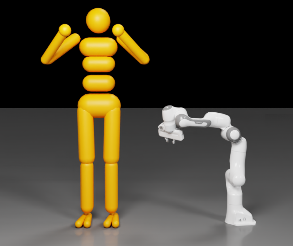
The tree structure for the arm is straightforward: The root is at the base on the ground plane, and revolute joints connect the different links up to the manipulator, where the tree has its only branch to connect the two gripper parts to the arm through prismatic (i.e. linear) joints.
The ragdoll also has a tree structure: For example, we can choose the head to be the root, and connect the torso to it with a spherical joint, which in turn uses spherical joints to attach the arms, and so on. The tree structure would be broken if the ragdoll was handcuffed such that the hands, arms, and torso form a loop.
Floating and Fixed-Base
There is a difference between the two articulation examples: The ragdoll is a floating articulation which means the root (e.g. the head) may move freely in space.
The robot arm is a fixed-base articulation: Its root or base is fixed to the world frame. The fixed-base property can be set with a flag on the articulation at creation. Setting this flag is advantageous over constraining the root link using a Fixed Joint because the immoveable property of the root link is solved perfectly.
Closing Loops
While articulations natively only support tree-structures, it is possible to create loops in the articulation by adding rigid-body Joints between articulation links. For example, we could tie the ragdoll’s hands together by adding a Distance Joint between the two hand spheres.
Reduced-Coordinates and Comparison to Rigid Bodies
The links that make up an articulation are actors like rigid bodies, but they are simulated as a unit. One of the differences between a link and a rigid body is that it is not possible to set a link’s global pose or velocity directly. This is due to the reduced-coordinate representation: The pose of a link is determined recursively through the pose of its parent link and the position of the joint connecting it to the parent (velocities are analogous). For the same reason, links cannot be kinematic. You may find more details about reduced coordinates below.
The articulation links also do not have individual sleep states or solver iteration counts because they are simulated as a unit in the articulation. Those properties are set on the articulation instead. For the same reason, the links do not support force thresholding.
Otherwise, articulation links can be treated as rigid bodies; for example, they use the same mass and collision-shape setup API, or we can apply a spatial force to them, or we can query their world pose and velocity (querying is ok, setting is not). In particular, links are also compatible with rigid-body Joints that can be used to close loops.
Performance-wise, the simulation cost is generally proportional to the number of degrees of freedom, rather than the number of links (assuming few contacts that need resolving). Therefore, in common robotics applications, where most joints have 0-1 degrees of freedom, the simulation cost of reduced-coordinate articulations is often lower than using rigid-bodies with joints.
Creating an Articulation
First, create the articulation actor without links:
PxArticulationReducedCoordinate* articulation = physics.createArticulationReducedCoordinate();
Set the articulation to be fixed-base, if applicable, and any other optional configuration options (see the API doc of PxArticulationFlag and PxArticulationReducedCoordinate for more information):
articulation->setArticulationFlag(PxArticulationFlag::eFIX_BASE, true);
articulation->setSolverIterationCounts(minPositionIterations, minVelocityIterations);
articulation->setMaxCOMLinearVelocity(maxCOMLinearVelocity);
// etc.
Then add links one by one, each time specifying a parent link (NULL for the parent of the initial link), and the pose of the new link:
PxArticulationLink* link = articulation->createLink(parent, PxTransform());
PxRigidActorExt::createExclusiveShape(*link, linkGeometry, material);
PxRigidBodyExt::updateMassAndInertia(*link, 1.0f);
Note that the initial poses of the child links may be set to arbitrary transforms since the child link poses are computed from the base link pose and the joint positions when they are set to their initial values via the cache, see PxArticulationCache. Hence one can just pass an identity PxTransform.
Each time a link is created beyond the first, a PxArticulationJoint is created between it and its parent. Specify the joint frames for each joint, in exactly the same way as for a rigid-body PxJoint:
PxArticulationJointReducedCoordinate* joint = link->getInboundJoint();
joint->setParentPose(parentAttachment);
joint->setChildPose(childAttachment);
and configure the joint type and motion - here an example of a joint with a limited motion range:
joint->setJointType(PxArticulationJointType::eREVOLUTE);
// revolute joint that rotates about the z axis (eSWING2) of the joint frames
joint->setMotion(PxArticulationAxis::eSWING2, PxArticulationMotion::eLIMITED);
PxArticulationLimit limits;
limits.low = -PxPiDivFour;  // in rad for a rotational motion
limits.high = PxPiDivFour;
joint->setLimitParams(PxArticulationAxis::eSWING2, limits);
Note how the axis must be specified consistently for both setting the motion and limit. In addition to limits, you may add a joint drive (i.e. motor):
PxArticulationDrive posDrive;
posDrive.stiffness = driveStiffness;                      // the spring constant driving the joint to a target position
posDrive.damping = driveDamping;                        // the damping coefficient driving the joint to a target velocity
posDrive.maxForce = actuatorLimit;                        // force limit for the drive
posDrive.driveType = PxArticulationDriveType::eFORCE;    // make the drive output be a force/torque (default)
// apply and set targets (note again the consistent axis)
joint->setDriveParams(PxArticulationAxis::eSWING2, posDrive);
joint->setDriveVelocity(PxArticulationAxis::eSWING2, 0.0f);
joint->setDriveTarget(PxArticulationAxis::eSWING2, targetPosition);
You may also set joint friction, armature, etc; see the API doc of PxArticulationJointReducedCoordinate for details. At creation, you can also add Articulation Tendons or Articulation Link Sensors:
PxArticulationSensor* sensor = articulation->createSensor(link, sensorPose);
// setup sensor
PxArticulationFixedTendon* fixedTendon = articulation->createFixedTendon();
// setup tendon
Finally, add the articulation to the scene (see caveat below about changing articulation topology after scene insertion):
scene.addArticulation(*articulation);
Changing the Topology of an Articulation that is in a Scene
In order to allow for pre-computing and optimization of simulation data, it is not possible to make changes to an articulation that change its topology after the articulation has been added to the scene. Topological changes include:
If you need to make topology changes, simply remove and re-add the articulation to the scene:
scene->removeArticulation(*articulation);
// make topology changes
scene->addArticulation(*articulation);
The articulation state (i.e. pose and velocities) is preserved through the remove and re-add cycle, so you do not have to store and reapply the state. In case of link removal, the corresponding joint state is removed as well; the state of joints of new links may be set with PxArticulationJointReducedCoordinate::setJointPosition() and PxArticulationJointReducedCoordinate::setJointVelocity() or the PxArticulationCache. Note that any changes to the articulation topology, in particular changes affecting degrees-of-freedom, typically require recreating the articulation’s PxArticulationCache and recomputing low-level indices to the cache.
Articulations and Sleeping
Like rigid dynamic objects, articulations are put into a sleep state if their energy falls below a certain threshold for a period of time. In general, all the points in the section Sleeping apply to articulations as well. In particular, articulations can only go to sleep if each individual articulation link fulfills the sleep criteria, analogous to jointed rigid-bodies.
Articulation Joints
The PxArticulationJointReducedCoordinate provides an interface that is similar to the PxD6Joint interface for rigid-body joints. However, it incurs certain limitations. By default, all axes are locked and the joint type is undefined. The joint types are:
PxArticulationJointType::eFIX- a fixed joint with zero degrees of freedom (DOF)PxArticulationJointType::ePRISMATIC- a prismatic (sliding) joint with one DOFPxArticulationJointType::eREVOLUTE- a revolute (hinge) joint with one DOF whose position is automatically wrapped at +/- 2pi.PxArticulationJointType::eREVOLUTE_UNWRAPPED- same as a revolute, but without position wrappingPxArticulationJointType::eSPHERICAL- a spherical (ball-in-socket) joint with two to three DOFs
See Creating an Articulation for setup example code.
Articulation joints are not breakable like rigid-body joints. Furthermore, note that spherical joints are a special case: while it is technically possible to configure a spherical joint to only have one DOF, you should use a revolute joint instead for performance. When there are two or more degrees of freedom unlocked, rotational motion is integrated by rotating by decomposed quaternions rather than by Euler angles to avoid gimbal lock. However, this technique can lead to rotational axis drift, which is corrected by additional constraints in the simulation, which could lead to slight movement on the remaining locked rotational axis.
Articulation Joint Drives
In addition, a drive may be added to a joint. As with limits, this is defined on a per-axis basis. The drives operate analogous to a PD controller (see implementation note below) and have two terms: stiffness and damping. Stiffness controls how strongly the drive drives towards a target joint position/angle and damping controls how strongly the joint drives towards a target velocity. Let’s consider again the sample setup code in Creating an Articulation:
PxArticulationDrive posDrive;
posDrive.stiffness = driveStiffness;                      // the spring constant driving the joint to a target position
posDrive.damping = driveDamping;                          // the damping coefficient driving the joint to a target velocity
posDrive.maxForce = actuatorLimit;                        // force limit for the drive
posDrive.driveType = PxArticulationDriveType::eFORCE;     // make the drive output be a force/torque (default)
// apply and set targets (note again the consistent axis)
joint->setDriveParams(PxArticulationAxis::eSWING2, posDrive);
joint->setDriveVelocity(PxArticulationAxis::eSWING2, targetVelocity);
joint->setDriveTarget(PxArticulationAxis::eSWING2, targetPosition);
With these parameters, the joint drive pushes the joint position towards targetPosition [rad] and the joint velocity toward targetVelocity [rad/s]. Assuming that the scene units are (SI) meters, the drive output is a torque in [Nm], the driveStiffness gain on position is in [Nm/rad], and the driveDamping gain on velocity is in [Nm/(rad/s)].
If the driveType is instead set to PxArticulationDriveType::eACCELERATION, the drive output is a joint acceleration, which can be useful to obtain behavior that is independent of the mass and inertia of the links. For an acceleration drive, the driveStiffness gain has units [rad/s^2 / rad], and driveDamping is in [rad/s^2 / (rad/s)].
An key articulation flag related to drives is PxArticulationFlag::eDRIVE_LIMITS_ARE_FORCES: If it is set, the forceLimit above refers to a force/torque (e.g. N and Nm), and, otherwise, to an impulse (force * dt, or torque * dt). The limit applies to both force- and acceleration-type drives.
The joint drive can be made into a velocity drive tracking targetVelocity by setting driveStiffness to zero and an appropriately tuned driveDamping. By default, the target velocity of the drive is set to 0 [rad/s], so a nonzero damping parameter results in the drive being an PD controller where the P gain, i.e. the stiffness, acts on the position error and the D gain, i.e. the damping, acts on the derivative of the position error, i.e. opposing the joint velocity.
It is possible to retrieve the constraint forces (i.e. drive, joint limits, and joint friction) applied by the solver, see PxArticulationCacheFlag::eJOINT_SOLVER_FORCES and PxArticulationFlag::eCOMPUTE_JOINT_FORCES.
Note
An important implementation detail is that the drives are implicit, i.e. the position and velocity constraints imposed by the drive that the solver iterates on are with respect to the end of the time step, and not, as usual (in engineering) implemented as an explicit, constant-during-time-step drive force calculated from the gains and the joint position and velocity at the beginning of the time step. The nice property of the implicit formulation is that it can handle very large gains without necessarily causing joint state instability or oscillations. Of course, for low gains and small enough time steps, the implicit and explicit drive dynamics will be practically identical.
Joint Positions and Velocities
Reduced-coordinate articulations internally keep track of scalar joint positions, velocities, and accelerations, with one entry corresponding to each degree of freedom (DOF). Joint position represents the relative offset between a parent and child link, and their corresponding joint frames in particular, along/around a DOF. If it is a rotational axis, the joint position represents an angle in radians. If it is a translational axis, the joint position represents a distance in whatever units the simulation is being performed in. Similarly, joint velocities are in radians/s or distance/s, for a rotational and linear DOF.
The joint positions determine the links’ poses: The root link’s world space pose provides a reference frame from which the poses for all other links in the articulation are calculated from the joint positions. This ensures that there cannot be any joint separation or offsets in locked axes.
The caveat with this approach is that it is not possible to directly update the pose of links in an articulation because this new transform could violate locked axes or could differ from the joint position. Instead, it is necessary to update the joint positions, which triggers new link poses to be computed. This ensures that the internal data from which poses are computed is consistent at all times. See PxArticulationCache below for more information on how to set/read joint positions and other internal data of the articulations.
Link velocities and joint velocities share a similar relationship. A link’s world-space velocity is derived from the world-space velocity of its parent link and the current joint velocity. This means that the root link stores a world-space velocity and all other links’ velocities are computed by propagating this velocity and the respective joint velocities through the articulation. As such, it is not possible to directly set the velocity of links in an articulation. Instead, it is necessary to modify the root and joint velocities from which the links’ velocities are calculated. It is legal to apply world-space forces on links. These will be propagated through the articulation as part of forward dynamics.
Note
Just like rigid bodies, all queries regarding link velocity and acceleration report the respective quantities in the world frame and with the links’ center of mass as reference point (and not the actor frame’s origin). However, also like rigid bodies, pose is reported with respect to the actor frame.
Reduced-coordinate articulation textbooks, e.g. Rigid Body Dynamics Algorithms by Roy Featherstone, use spatial accelerations to describe the rigid-body, i.e. link accelerations. PhysX does not report spatial accelerations, but classical, i.e. body-fixed accelerations.
PxArticulationCache
Direct access to joint positions, velocities and forces, and other internal data that controls a reduced-coordinate articulation is provided through the PxArticulationCache class and the corresponding API in PxArticulationReducedCoordinate.
Create a cache as follows after you inserted the articulation into a scene:
PxArticulationCache* cache = articulation->createCache();
The cache is constructed specifically for the g articulation and contains the exact memory needed to store data about that articulation. It cannot be shared between different articulations unless they have the exact same structure. Similarly, if the properties of an articulation change (e.g. a link or force sensor is added/removed, or degrees of freedom are changed), it is necessary to release the cache and recreate it.
Once a cache has been created, it may be used to read articulation data by copying the data into the cache. In this case, all data is copied to the cache, but the copy may be filtered to data of interest with PxArticulationCacheFlag:
articulation->copyInternalStateToCache(*cache, PxArticulationCacheFlag::eALL);
Since the data in the cache is a copy of the articulation data, any modifications to the cache data do not alter the internal state of the articulation that copied the data to the cache. In order to update the internal state of the articulation, it is necessary to apply the cache, i.e. copy the data back to the articulation. In this example, we apply, i.e. copy just the joint positions:
articulation->applyCache(*cache, PxArticulationCacheFlag::ePOSITION);
Note that this will cause the link poses to be updated based on the newly set joint positions, and it is not legal to copy to or apply a cache while the simulation is running.
A cache stores sufficient information to be able to record the state of an entire articulation at a snapshot in time and then reset the articulation back to that state. It is legal to create and maintain multiple articulation caches for a given articulation.
A cache further provides access to the root link’s state, including transform, velocities and accelerations. See PxArticulationCache for further articulation data that may be accessed via cache.
Simple operations like zeroing the joint velocities can be done with the following code snippet:
PxMemZero(cache->jointVelocity, sizeof(PxReal) * articulation->getDofs());
articulation->applyCache(*cache, PxArticulationCacheFlag::eVELOCITY);
In addition to setting joint positions and velocities, it is possible to interact with the articulation through the application of joint forces/torques, which behave like an actuator, or by applying external forces to the links directly.
Cache Indexing
The data in the cache is stored in a specific internal low-level order that facilitates propagation through the articulation. The order imposed by the low-level indices may be different from the order in which the links and joints were originally added to the articulation. Therefore, the user must:
use a link’s low-level index
PxArticulationLink::getLinkIndex()for link-data indexing, e.g.PxArticulationCache::externalForces;use a link force sensor’s
PxArticulationSensor::getIndex()for spatial sensor force indexing;calculate the low-level degree-of-freedom (DOF) data indices by summing the joint DOFs in the order of the links’ low-level indices:
Low-level link index:   | link 0 | link 1 | link 2 | link 3 | ... | <- PxArticulationLink::getLinkIndex()
Link inbound joint DOF: | 0      | 1      | 2      | 1      | ... | <- PxArticulationLink::getInboundJointDof()
Low-level DOF index:    | -      | 0      | 1, 2   | 3      | ... |
The root link always has low-level index 0 and always has zero inbound joint DOFs. The link DOF indexing follows the order in PxArticulationAxis::Enum. For example, assume that low-level link 2 has an inbound spherical joint with two DOFs: eSWING1 and eSWING2 (and, in particular, eTWIST is locked with PxArticulationMotion::eLOCKED). The corresponding low-level joint DOF indices are therefore 1 for eSWING1 and 2 for eSWING2.
Snippet: Calculate the low-level DOF indices for an articulation:
const PxU32 nbLinks = art->getNbLinks();
std::vector<PxArticulationLink*> links(nbLinks, nullptr);
// The links vector is in the order that the links are added to the articulation using createLink.
// However, the index in links[index] and the low-level index links[index].getLinkIndex() may differ
// depending on the articulation.
art->getLinks(links.data(), nbLinks, 0);
std::vector<PxU32> dofStarts(nbLinks, 0);
dofStarts[0] = 0;  // The root link never has an incoming articulation joint

// Put DOF counts into dofStarts in low-level index order
for(PxU32 i = 1; i < nbLinks; ++i)
{
    PxU32 lowLevelIndex = links[i]->getLinkIndex();
    PxU32 dofs = links[i]->getInboundJointDof();
    dofStarts[lowLevelIndex] = dofs;
}

// Calculate DOF index offsets per low-level link index:
PxU32 count = 0;
for(PxU32 i = 1; i < nbLinks; ++i)
{
    PxU32 dofs = dofStarts[i];
    dofStarts[i] = count;
    count += dofs;
}
Consider again the spherical joint described above and that it is the incoming joint of PxArticulationLink* link. We can set the position of the joint’s eSWING2 DOF with:
PxU32 jointSwingTwoIndex = 1;
cache->jointPosition[dofStarts[link->getLinkIndex()] + jointSwingTwoIndex] = newJointPosition;
In addition to reading and writing joint DOF data, the cache is used to read and write data for computations that can be performed using reduced coordinate articulations, for example, inverse dynamics and Jacobian matrix computations.
Articulation Tendons
Tendons create constraints within articulations. There are two types: Fixed and Spatial.
Fixed Tendons
Fixed tendons impose constraints on joint positions. For example, a fixed tendon can be setup such that it imposes an equality constraint between a driven and a passive revolute joint. More details are available in the API documentation for PxArticulationFixedTendon.
Spatial Tendons
Spatial tendons impose distance constraints between attachment points on links. This allows, for example, modeling hydraulic actuators that can push and pull on links, artificial muscles in a biomimetic robot, or elastic-string-like mechanical components. More details are available in the API documentation for PxArticulationSpatialTendon.
Articulation Link Sensors
Sensors can be attached to articulation links in order to read out forces and torques acting on a link. For more details, refer to the API doc of PxArticulationSensor.
Note
The SDK team is reworking the specifications for the sensors together with robotics users, so the data that they report will change in a future release based on the updated specifications.
Best Practices and Simulation Detail
Stability
The reduced coordinate articulations are suitable for use in games to simulate humanoids, i.e. ragdolls. However, introducing velocity clamps or damping may be required to ensure stability of the simulation at large angular velocities. The reason for this is the explicit integration of Coriolis and centrifugal forces. There are several options available to introduce damping and clamping by setting
rigid body velocity limits and damping; or
nonzero joint friction; or
adding a joint drive with nonzero damping
adding center-of-mass (COM) limits to the articulation
Inverse Dynamics, Jacobian and other Utility Computations
The reduced coordinate articulations offer inverse dynamics functionality in addition to forward dynamics used in simulation. This is a suite of utility functions to compute the joint forces required to counteract gravity, Coriolis/centrifugal force, external forces, and contacts/constraints. Furthermore, there are utility functions to compute kinematic Jacobians, the mass matrix, and the coefficient matrix and lambda values.
The following descriptions assume knowledge of inverse dynamics concepts.
Preparing the Articulation for Inverse Dynamics Computations
Prior to performing any inverse dynamics calculations, it is necessary to ensure that constant joint data has been computed. In order to do this, follow the steps
Set articulation pose (joint positions and base transform) via articulation cache and applyCache.
Depending on method: Setup base link velocity, and computation input values in cache.
Call inverse dynamics computation method, e.g.
PxArticulationReducedCoordinate::computeJointForce().
Converting From and To Reduced Coordinate Joint DOF Coordinates
The inverse dynamics functions operate on an articulation and a PxArticulationCache. The majority of properties in PxArticulationCache are stored in a reduced/generalized coordinate space, where one entry corresponds to a degree of freedom. To simplify working in this space, PhysX provides the following methods to pack and unpack data to convert between reduced/generalized and maximal coordinates.
Indexing: Indexing into the link maximum joint DOF data is via the link’s low-level index minus 1 (the root link is not included), and the reduced-coordinate DOF data follows the cache indexing convention, see Cache Indexing.
Example: Unpack a reduced-coordinate joint position of a fixed-base 1-DOF pendulum with a revolute joint with a free eSWING2 (z) motion:
PxReal maximalJointPositions[6] = { 0.0f };
PxReal reducedJointPosition = 0.5f;
articulation->unpackJointData(&reducedJointPosition, maximalJointPositions);
// Result: maximalJointPositions[PxArticulationAxis::eSWING2] is equal to 0.5f, and all other elements are 0.0f
Example: Pack maximal joint positions of a fixed-base 1-DOF pendulum with a revolute joint with a free eSWING2 (z) motion:
PxReal maximalJointPositions[6] = { 0.0f };
maximalJointPositions[PxArticulationAxis::eSWING2] = 0.5f;
PxReal reducedJointPosition = 0.0f;
articulation->packJointData(maximalJointPositions, &reducedJointPosition);
// Result: reducedJointPosition is equal to 0.5f
Compute Generalized Gravity Force
With:
articulation->computeGeneralizedGravityForce(*cache);
we can compute the joint DOF forces required to counteract gravitational forces for the given articulation pose. The joint forces returned are determined purely by gravity for the articulation in the current joint and base pose, i.e. external forces, joint velocities, and joint accelerations are set to zero. In addition, any joint drives are not considered in the computation. The computed forces correspond to the (joint-space) G(q) term in a robotics manipulator equation.
Inputs: Articulation pose (joint positions and base transform).
Outputs: Joint forces to counteract gravity (in cache).
Example: Calculate holding torque to apply at a pendulum’s pivot when it is perpendicular to the gravity vector:
// set articulation pose to evaluate gravity forces at
cache->jointPosition[0] = PxPiDivTwo; // Set pendulum to be perpendicular to gravity
pendulumArticulation->applyCache(*cache, PxArticulationCacheFlag::ePOSITION);

// prepare common articulation data in newly set pose for inverse dynamics calculation
pendulumArticulation->commonInit();
pendulumArticulation->computeGeneralizedGravityForce(*cache);

PxReal massPendulum = 1.0f;        // [kg]
PxReal distancePivotToCOM = 1.0f;  // [m]
PxReal gravityMagnitude = 10.0f;   // [m / s^2]
PxReal analyticHoldingTorque = massPendulum * distancePivotToCOM * gravityMagnitude;  // [N * m]
PxReal computedHoldingTorque = cache->jointForce[0];  // will be equal to analyticHoldingTorque = 10.0f

// we can now directly apply the computed torque; for example to gravity-compensate a simulated robot arm.
// make sure pendulum is at rest before simulation. Force is still set in cache from computation above.
cache->jointVelocity[0] = 0.0f;
pendulumArticulation->applyCache(*cache, PxArticulationCacheFlag::eVELOCITY | PxArticulationCacheFlag::eFORCE);

// simulate a single step
runSim(1);

// read out post-simulation joint velocity
art->copyInternalStateToCache(*cache, PxArticulationCacheFlag::eVELOCITY);
PxReal postSimVel = cache->jointVelocity[0];  // will be zero
Compute Coriolis Joint Forces
With:
articulation->computeGeneralizedExternalForce(*cache);
we can compute the joint DOF forces required to counteract Coriolis and centrifugal forces for the given articulation state. The joint forces returned are determined purely by the articulation’s state; i.e. external forces, gravity, and joint accelerations are set to zero. Joint drives and potential damping terms, such as link angular or linear damping, or joint friction, are also not considered in the computation. The computed forces correspond to the (joint-space) C(q,qdot) term in a robotics manipulator equation.
Inputs: Articulation state (joint positions and velocities (in cache), and base transform and spatial velocity).
Outputs: Joint forces to counteract Coriolis and centrifugal forces (in cache).
To compute the joint force required to counteract Coriolis and centrifugal force, we must first provide the joint velocities of the articulation because coriolis/centrifugal forces are dependent on those values. In this example, we extract the velocities from the articulation before computing coriolis/centrifugal force:
articulation->copyInternalStateToCache(*cache, PxArticulationCache::eVELOCTY);
articulation->computeCoriolisAndCentrifugalForce(*cache);
Example: Calculate joint torques to keep a double pendulum’s joint accelerations zero when the first link is rotating with 1 rad/s around the fixed pivot and with the second link perpendicular to the first (so that a centrifugal force has to be countered):
// initial joint states:
cache->jointPosition[0] = 0.0f;        // does not matter
cache->jointPosition[1] = PxPiDivTwo;  // perpendicular to first link
cache->jointVelocity[0] = 1.0f;        // rotate at 1 rad/s
cache->jointVelocity[1] = 0.0f;        // at rest relative to first link

// set articulation state (velocity not required for computation, but for later simulation from given state):
doublePendulum->applyCache(*cache, PxArticulationCacheFlag::ePOSITION | PxArticulationCacheFlag::eVELOCITY);

// prepare common articulation data for inverse dynamics calculation:
doublePendulum->commonInit();

// compute centrifugal torque (the joint velocities in the cache are used for the computation here)
doublePendulum->computeCoriolisAndCentrifugalForce(*cache);
PxReal centrifugalForce = cache->jointForce[1];

// compute gravity compensation as well to keep acceleration zero:
doublePendulum->computeGeneralizedGravityForce(*cache);

// add back centrifugal torque
cache->jointForce[1] += centrifugalForce;

// apply torques at joints
doublePendulum->applyCache(*cache, PxArticulationCacheFlag::eFORCE);

// run one sim step and get post-sim joint velocities:
runSim(1);
doublePendulum->copyInternalStateToCache(*cache, PxArticulationCacheFlag::eVELOCITY);
PxReal postSimVelOne = cache->jointVelocity[0];  // will be 1 rad/s
PxReal postSimVelTwo = cache->jointVelocity[1];  // will be 0 rad/s
Compute Generalized External Force
With:
articulation->computeGeneralizedExternalForce(*cache);
we can compute the joint DOF forces required to counteract external spatial forces applied to articulation links. Only the external forces and the current articulation pose are considered in the calculation.
The external spatial forces are with respect to the links’ centers of mass, and not the actor’s origin.
Inputs: External forces on links (in cache), articulation pose (joint positions + base transform).
Outputs: Joint forces to counteract the external forces (in cache).
Example: Compute joint torque at pendulum articulation pivot when spatial force is applied to the pendulum center of mass:
// set pendulum pose
// the angle is in +Z relative to upright where the pendulum coincides with +Y, and the pivot is at the origin.
PxReal pendulumAngle = PxPiDivFour;
cache->jointPosition[0] = pendulumAngle;
pendulum->applyCache(*cache, PxArticulationCacheFlag::ePOSITION);

// prep common articulation data for given pose for inverse dynamics computation
pendulum->commonInit();

// Define the spatial force to apply to the pendulum
// Note that this spatial force is defined with respect to the center of mass of the link
// which may or may not coincide with the actor frame origin (@see PxRigidBody::getCMassLocalPose)
PxSpatialForce force = PxSpatialForce();
force.force = PxVec3(1.0f, 0.0f, 0.0f);  // acts on center of mass!
force.torque = PxVec3(0.0f, 0.0f, 1.0f);

PxArticulationLink* pendulumLink = nullptr;
// getLinks is indexed in order that the links were added to the articulation
PxU32 linkIndex = 1u;
PxU32 bufferSize = 1u;
pendulum->getLinks(&pendulumLink, bufferSize, linkIndex);
// external forces are indexed by low-level link index
// (for this simple articulation the low-level and getLinks indices will be equal)
cache->externalForces[pendulumLink->getLinkIndex()] = force;

pendulum->computeGeneralizedExternalForce(*cache);

// force in +X results in + counter torque and spatial torque in - counter torque
PxReal analyticCounterTorque = PxCos(pendulumAngle) * distancePivotToCOM * force.force.x - force.torque.z;
PxReal computedCounterTorque = cache->jointForce[0];

// analytic and computed are equal
Compute Joint Accelerations
With:
articulation->computeJointAcceleration(*cache);
we can compute the joint accelerations for the given articulation state and joint forces, taking into account gravity. Joint drives and potential damping terms are not considered in the computation (for example, linear link damping or joint friction).
Inputs: Joint forces (in cache) and articulation state (joint positions and velocities (in cache), and base transform and spatial velocity).
Outputs: Joint accelerations (in cache).
Example: Compute joint accelerations at pendulum articulation pivot with and without applying a joint force:
// calculate pendulum inertia for computations below:
PxReal inertiaAtCOM = distancePivotToCOM * distancePivotToCOM * mass / 3.0f;
PxReal inertiaAtPivot = inertiaAtCOM + distancePivotToCOM * distancePivotToCOM * mass;

// Case 1: Pendulum perpendicular to gravity and zero input torque: Pivot acceleration will be due to gravity.
cache->jointPosition[0] = PxPiDivTwo;  // gravity will result in a positive angular acceleration
pendulum->applyCache(*cache, PxArticulationCacheFlag::ePOSITION);

// prepare articulation data for the computation
pendulum->commonInit();

cache->jointForce[0] = 0.0f;  // only consider acceleration due to gravity:
// For a more complex articulation than this simple example pendulum, the jointVelocity in the cache would have
// to be set for the computation of joint accelerations due to Coriolis terms.

pendulum->computeJointAcceleration(*cache);

PxReal torqueDueToGravityAtPivot = gravityMagnitude * mass * distancePivotToCOM;
PxReal analyticAcceleration = torqueDueToGravityAtPivot / inertiaAtPivot;
PxReal computedAcceleration = cache->jointAcceleration[0];

// analytic and computed are equal

// Case 2: Apply a torque to cancel the gravitational joint acceleration:
cache->jointForce[0] = -torqueDueToGravityAtPivot;  // 1 Nm input

// running computation with same articulation pose as Case 1, so no need to call commonInit again.
pendulum->computeJointAcceleration(*cache);
analyticAcceleration = 0.0f;
computedAcceleration = cache->jointAcceleration[0];

// analytic and computed are equal
Compute Joint Forces
With:
articulation->computeJointForce(*cache);
we can compute the joint forces required to achieve desired joint DOF accelerations for the given articulation state, not considering gravity. Joint drives and potential damping terms are not considered in the computation (for example, linear link damping or joint friction).
This method, together with computeGeneralizedGravityForce, can be used to calculate feed-forward joint forces to apply to follow a reference joint-space trajectory using feedback control.
Inputs: Joint accelerations (in cache) and articulation state (joint positions and velocities (in cache), and root transform and spatial velocity).
Outputs: Joint forces (in cache).
Example: Compute joint forces at pendulum articulation pivot in order to achieve a desired angular acceleration:
// calculate pendulum inertia for computations below:
PxReal inertiaAtCOM = distancePivotToCOM * distancePivotToCOM * mass / 3.0f;
PxReal inertiaAtPivot = inertiaAtCOM + distancePivotToCOM * distancePivotToCOM * mass;

// Pendulum angle will not matter because gravity is not considered in the computation
// so directly prepare articulation data for the computation
pendulum->commonInit();

PxReal targetAcceleration = 1.0f;  // rad/s^2
cache->jointAcceleration[0] = targetAcceleration;
// For a more complex articulation than this simple example pendulum, the cache jointVelocity member would have
// to be set for the computation of joint accelerations due to Coriolis terms

pendulum->computeJointForce(*cache);

PxReal analyticTorque = targetAcceleration * inertiaAtPivot;
PxReal computedTorque = cache->jointForce[0];

// analytic and computed are equal
Generalized Mass Matrix
With:
articulation->computeGeneralizedMassMatrix(*cache);
We can compute the generalized mass matrix, which represents the joint-space inertia of the articulation and can be used to convert joint accelerations into joint forces/torques, i.e. forces = massMatrix * accelerations. The indexing into the matrix follows the low-level joint DOF indexing, see Cache Indexing.
Inputs: Articulation pose (joint positions and base transform).
Outputs: The generalized mass matrix (in cache).
Loop Joints, Coefficient Matrix, and Lambda Constraint Impulses
Articulations are tree structures and do not support closed loops natively. PhysX can simulate closed loop systems by the use of joints. Additionally, contacts between links and other rigid bodies (e.g. the ground) can form loops if more than one link is in contact. These joints and contacts are solved by the rigid body solver during PhysX simulation, but it is often desirable to factor these constraints into inverse dynamics.
To facilitate this, PhysX provides a mechanism to register loop constraints with the articulation:
PxJoint* joint = ...;

articulation->addLoopJoint(joint);

articulation->removeLoopJoint(joint);
In order to represent contacts, use PxContactJoint: This is a new addition specifically for inverse dynamics that represents a contact as an extension to the joint system. Currently, the following features are restricted to the use of PxContactJoint.
Inverse dynamics provides functionality to calculate the coefficient matrix. This matrix is an NxM matrix, where N is the number of degrees of freedom in the articulation and M is the number constraint rows. This matrix represents the joint force caused by a unit impulse applied to each constraint:
PxU32 coefficientMatrixSize = articulation->getCoefficentMatrixSize();
PxReal* coefficientMatrix = new PxReal[coefficientMatrixSize];
cache->coefficientMatrix = coefficientMatrix;
articulation->computeCoefficientMatrix(*cache);
The coefficient matrix can be used to convert a set of lambda values (impulses applied by the respective constraints) into a set of joint forces to counteract these impulses. However, the lambda values are only known after a frame’s simulation occurs, so it may be necessary to know these lambda values before they are applied in the solver. However, even if these lambda values are known ahead-of-time, applying a counteracting force may not yield the desired results because the act of applying additional forces on the joints may influence the lambda values, resulting in a different set of joint forces.
In order to overcome this feedback-loop, inverse dynamics provides a function to compute the lambda values for the loop constraints, assuming that the joint forces required to counteract these lambdas are also applied. This technique is an iterative process that converges on a stable set of joint forces.
First, we must allocate sufficient space for the lambda values:
PxReal* lambda = new PxReal[articulation->getNbLoopJoints()];
cache->lambda = lambda;
In order to compute the lambda values, we need to have two caches: one to store the initial state, and one to calculate the final state:
PxArticulationCache* initialState = articulation->createCache()
articulation->copyInternalStateToCache(*initialState, PxArticulationCache::eALL);
Now we can compute the joint forces. In addition, we must compute the internal and external joint forces caused by gravity and Coriolis/centrifugal force to ensure that we converge on a result that will match the forward dynamics. The joint forces for internal/external accelerations can be calculated using the methods outlined earlier. The method is iterative and terminates either after reaching convergence or when a maximum number of iterations is run (in this case 200). The resulting joint forces are in cache.jointForce:
const PxU32 maxIterations = 200;
bool converged = articulation->computeLambda(*cache, *initialState, jointForces, maxIterations);
Jacobian
The Jacobian matrix is an important concept to roboticists. Multiplication with the Jacobian matrix maps the joint space velocities of the robot to world-space link velocities. The Jacobian matrix of an articulation can be computed using:
PxU32 nRows;
PxU32 nCols;
articulation->computeDenseJacobian(*cache, nRows, nCols);
This will write the Jacobian matrix to cache.denseJacobian; and the dimensions of the matrix are written to the two unsigned integers. Note that the Jacobian matrix is a sparse triangular matrix, so such an explicit dense representation is in general not an optimal use of memory. PhysX does not use this representation internally.
The spatial link velocities that the matrix maps to are with respect to the center of mass (COM) of the links, and are stacked [vx; vy; vz; wx; wy; wz], where vx and wx refer to the linear and rotational velocity in world X, respectively.
- Indexing:
Links, i.e. rows are in order of the low-level link indices (minus one if PxArticulationFlag::eFIX_BASE is true), see PxArticulationLink::getLinkIndex().
DOFs, i.e. column indices correspond to the low-level DOF indices, see Cache Indexing.
Example: Jacobian of a 1-DOF, single-link pendulum:
// setup perpendicular to gravity (-g * eY), and pointing in -eX direction away from pivot
cache->jointPosition[0] = PxPiDivTwo;
pendulum->applyCache(*cache, PxArticulationCacheFlag::ePOSITION);

PxU32 nRows = 0u;
PxU32 nCols = 0u;
pendulum->computeDenseJacobian(*cache, nRows, nCols);

// nRows will be equal to 6, as the fixed-base articulation has a single free link
// nCols will be equal to 1, as the pendulum has a single degree of freedom

// for a given joint velocity w in eZ and the given pendulum angle of 90deg,
// the spatial velocity of the pendulum only has two nonzero elements:
// vy = -w * distancePivotToCOM  <- because the spatial velocity is with respect to the COM of the pendulum
// wz = w   <- trivially the rotational velocity of the pivot joint
// The Jacobian is the partial derivative of the spatial velocity with respect to w, so the matrix will be:
// Jac[0, 0] = dvx / dw = 0
// Jac[1, 0] = dvy / dw = -distancePivotToCOM
// Jac[2, 0] = dvz / dw = 0
// Jac[3, 0] = dwx / dw = 0
// Jac[4, 0] = dwy / dw = 0
// Jac[5, 0] = dwz / dw = 1

// this is overkill for this simple articulation but shows how to calculate the row index for a more
// complex fixed-base articulation. Not done here, but the user in general has to follow the snippet in the
// Cache Indexing section above in order to find the low-level DOF index.
PxArticulationLink* pendulumLink = nullptr;
PxU32 linkIndex = 1u;  // getLinks is indexed in order that the links were added to the articulation
PxU32 bufferSize = 1u;
pendulum->getLinks(&pendulumLink, bufferSize, linkIndex);

PxU32 dofColumn = 0; // relevant column is the 0-th one that corresponds to the single DOF of the pendulum
// -1 on the low-level link index as the fixed base link is not included
PxU32 vyRow = ((pendulumLink->getLinkIndex() - 1) * 6) + 1;
PxU32 wzRow = ((pendulumLink->getLinkIndex() - 1) * 6) + 5;
PxReal jac10 = cache->denseJacobian[nCols * vyRow + dofColumn];  // equal to -distancePivotToCOM
PxReal jac50 = cache->denseJacobian[nCols * wzRow + dofColumn];  // equal to 1
Data-Oriented Direct GPU API
The two PxScene methods PxScene::applyArticulationData() and PxScene::applyArticulationData() allow batch read/write access to the articulation simulation data on the GPU, where the data is copied from/to user GPU buffers. The API is only enabled if PxSceneFlag::eSUPPRESS_READBACK (and PxSceneFlag::eENABLE_GPU_DYNAMICS) are set on the scene and the broadphase type is set to GPU as well, i.e. PxBroadPhaseType::eGPU.
The user buffers must be sized based on maximal index and component counts over all articulations that are in the scene.Let maxGpuIndex and maxDofs be the maximal GPU index and dof counts over all articulations in the scene; see PxArticulationReducedCoordinate::getGpuArticulationIndex() and PxArticulationReducedCoordinate::getDofs(), respectively. Then, the buffer for reading/writing dof positions (PxArticulationGpuDataType::eJOINT_POSITION) must allocate memory for maxGpuIndex * maxDofs elements of PxReal, i.e. floats.
The indices provided to the apply and copy methods then correspond directly to dof data in this buffer, where the start of the dof data for an articulation with GPU index index is at index * maxDofs, and the per-articulation dof ordering follows the CPU cache Cache Indexing. The other data types are analogous, e.g. PxArticulationGpuDataType::eLINK_TRANSFORM requires memory for maxGpuIndex * maxLinks elements of PxTransform, where the per-articulation link indices can be determined by PxArticulationLink::getLinkIndex().
Note
Combining the direct GPU API with the CPU API for runtime simulation parameter updates may result in incorrect behavior due to stale transform data on the CPU.