Vehicles
Introduction
PhysX support for vehicles has been significantly reworked in 5.1. More specifically, a new system of flexible vehicle components has been introduced. Components may be mixed, matched and customised to create different types of vehicle that may be simulated at different levels of computational complexity.
It is straightforward to recreate all of the drive models that were implemented in the legacy classes PxVehicleNoDrive, PxVehicleDrive4W, PxVehicleDriveNW and PxVehicleDriveTank without further modification to any component maintained by the Vehicle SDK. The difference now is that users are not limited to these drive models but instead may reuse components maintained by the Vehicle SDK in conjunction with custom components to create entirely new types of vehicle.
The fundamental physical models employed by the Vehicle SDK are largely unchanged. A number of bug fixes and improvements, however, have been made along the way. Where possible, legacy implementation is provided as an alternative to the standard implementation of the new Vehicle SDK. These legacy components are clearly labelled and are marked as deprecated with a planned removal in a future release.
Mechanical Model
The PhysX Vehicle SDK models vehicles as collections of sprung masses, where each sprung mass represents a suspension line with associated wheel and tire data. These collections of sprung masses have a complementary representation as a rigid body whose mass, center of mass, and moment of inertia matches exactly the masses and coordinates of the sprung masses. This is illustrated below.
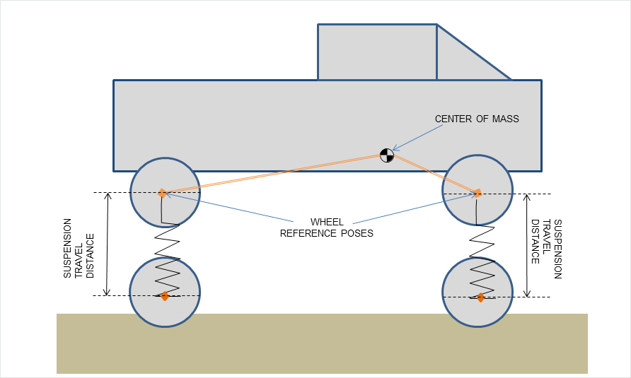
Figure 1a: Vehicle representation as a rigid body. Note that the wheel reference poses are specified relative to the rigid body center of mass.
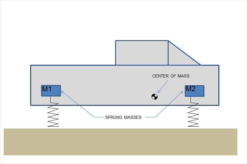
Figure 1b: Vehicle representation as a collection of sprung masses of mass M1 and M2.
The relationship between the sprung mass and rigid body vehicle representations can be mathematically formalized with the rigid body center of mass equations:
M = M1 + M2

0 = (M1 x X1 + M2 x X2)/(M1 + M2)
where M1 and M2 are the sprung masses; X1 and X2 are the sprung mass coordinates in the rigid body frame; and M is the rigid body mass.
The components of the PhysX Vehicle compute the suspension and tire forces using the sprung mass model and then forward integrate the aggregate of these forces applied to the vehicle’s rigid body representation.
The update of each vehicle begins with a scene query for each suspension in order to determine the road geometry plane under each wheel. The query begins at the pose of the wheel at maximum compression and casts downwards along the direction of suspension travel to the position of the wheel at maximum droop. This is shown in the diagram below.
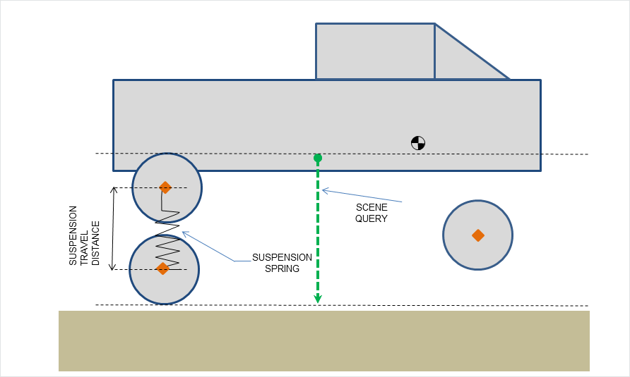
Figure 2: Suspension limits and geometry queries.
The suspension force from each elongated or compressed spring is computed and added to the aggregate force to be applied to the rigid body. Additionally, the suspension force is used to compute the load that is bearing down on the tire. This load is used to determine the tire forces that will be generated in the contact plane and then added to the aggregate force to be applied to the rigid body. The tire force computation actually depends on a number of factors including steer angle, camber angle, friction, wheel rotation speed, and rigid body momentum. The aggregated force of all tire and suspension forces is then applied to the vehicle’s rigid body and forward integrated. Integration with the PhysX scene is achieved by creating an PxRigidBody instance and setting its linear and angular velocities to be the values held by the vehicle’s rigid body. The PhysX scene forward integrates the geometry and momentum of the PxRigidBody instance and manages rigid body contacts that occur between the vehicle and the rest of the PhysX scene. The pose and momentum of the PxRigidBody instance is then passed to the vehicle’s rigid body for the next vehicle simulation step.
In addition to being collections of sprung masses, PhysX vehicles also support a variety of drive models. The center of the drive model is a torsion clutch, which couples together the wheels and the engine via forces that arise from differences in rotational speeds at both sides of the clutch. At one side of the clutch is the engine, which is powered directly from the accelerator pedal. The engine is modeled as a rigid body whose motion is purely rotational and limited to a single degree of rotational freedom. At the other side of the clutch are the gearing system, the differential and the wheels. The effective rotational speed of the other side of the clutch can be computed directly from the gearing ratio and the rotational speed of the wheels that are coupled to the clutch through the differential. This model naturally allows engine torques to propagate to the wheels and wheel torques to propagate back to the engine.
The data describing each component of the PhysX vehicle can be found in Section Tuning Guide.
Software Architecture
Overview
Vehicles are made of:
commands
parameters
states
C functions
components
component sequences.
Custom combinations of parameter, state and component allow different behaviours to be simulated with different simulation fidelities. For example, a suspension component that implements a linear force response with respect to its compression state could be replaced with one that imlements a non-linear response. The replacement component would consume the same suspension compression state data and would output the same suspension force data structure. In this example, the change has been localised to the component that converts suspension compression to force and to the parameterisation that governs that conversion. Another combination example could be the replacement of the tire component from a low fidelity model to a high fidelty model such as Pacejka. The low and high fidelity components consume the same state data (tire slip, load, friction) and output the same state data for the tire forces. Again, the change has been localised to the component that converts slip angle to tire force and the parameterisation that governs the conversion.
Commands
There are two types of command: universal commands that are applied to all vehicles and transmission commands that are unique to each vehicle type.
Vehicles are controlled by normalised parameters indicating the state of the throttle pedal, the brake pedal, the handbrake and the steering wheel. These are the universal commands that are common to all vehicle types supported by the Vehicle SDK. It is worth noting that the brake and the handbrake both apply brake torques to wheels. As a consequence, the brake and the handbrake are combined into an array of brake values. Each brake value in the array may be configured as a brake or as a handbrake by configuring brake response parameters for each type of brake. Alternatively, each brake value in the array may be used to simulate the left and right brake levers of a tank. The interpretation of any command, be that steering wheel or throttle or brake, depends on the sequence of components and functions that consume the commands.
Transmission commands are unique to each type of drive. For example, direct drive mode has a single command for forward, reverse or neutral gear. The gearing selected acts as a multiplier that is applied to the available drive torque before distributing torque to the driven wheels. Engine drive mode, on the other hand, has a command that either engages automatic gear or instantiates a gear change. It also has a clutch command that engages and disengages the clutch. Tank drive not only supports gear changes and clutch control but also has two thrust commands that simulate left and right thrust levers that distribute available drive torque to the wheels of the left and right tank tracks.
Universal commands are implemented with the following struct:
Transmission commands are implemented by the following structs:
Parameters
Parameters describe the configuration of the vehicle and the physics model employed. Examples are vehicle mass, wheel radius and suspension stiffness. Parameters remain constant throughout a single simulation step.
States
States describe the instantaneous dynamic state of a vehicle. Examples are engine revs, wheel yaw angle and tire slip angles. Each simulation step will update the state data of a vehicle.
C Functions
The Vehicle SDK ships with a maintained set of C functions. These functions are invoked by components to perform the computation required to update a vehicle.
Components
Components forward integrate the dynamic state of the vehicle, given command inputs, the previous vehicle state and the vehicle’s parameterisation. Components update dynamic state by invoking reusable C functions in a particular sequence. An example component is a rigid body component that forward integrates the linear and angular velocity of the vehicle’s rigid body given the instantaneous forces and torques of the suspension and tire states.
Components are typically designed to reflect human-level understanding of the constituent parts of a vehicle’s mechanical model. Tire force computation serves as an example. Computing a tire force involves a series of function calls to compute the tire slips and to convert the tire slips into forces. It makes sense to abstract this sequence of function calls into a single unit.
Each component is a sub-class of PxVehicleComponent, an interface class with a single pure virtual function:
virtual bool PxVehicleComponent::update(const PxReal dt, const PxVehicleSimulationContext& context) = 0;
Each component maintained by the Vehicle SDK implements the update() function and introduces one more pure virtual function. This virtual function gathers all of the command, parameter and state data required by the sequence of C functions that will be executed by the component. The idea here is that vehicles may employ any data layout, provided that layout can fulfil the requirements of the virtual function. This is discussed in more detail in Sections Vehicle Design Pattern and Parameter and State Data Layout. Custom components may follow this pattern or may directly store pointers and references to parameter and state data in the custom component class instances.
A vehicle update is performed by updating a sequence of components in a defined order.
Component Sequences
The pipeline of vehicle computation is a sequence of components that run in a defined order. For example, one component might compute the plane under the wheel by performing a scene query against the world geometry. The next component in the sequence might compute the suspension compression required to place the wheel on the surface of the hit plane. Following this, a subsequent component might compute the suspension force that arises from that compression. The rigid body component, as discussed in Section Mechanical Model, can then forward integrate the rigid body’s linear velocity using the suspension force.
The class PxVehicleComponentSequence allows component sequences to be defined and updated.
Components are added according to the order of execution:
PxVehicleComponentSequence sequence;
sequence.add(new ComponentBegin);
sequence.add(new ComponentMiddle);
sequence.add(new ComponentEnd);
Chains of subsequent components may be grouped together into sub-stepping groups within the component sequence. Each sub-stepping group of components will be updated in order an integer number of times with a timestep that reflects the number of updates. This allows small timesteps to be directed at the numerically stiffest parts of the simulation without the computational cost of simulating the entire pipeline at a small timestep. The following pseudo-code demonstrates a substepping group of two components ComponentMiddle1 and ComponentMiddle2 that will be updated 3 times per sequence update:
PxVehicleComponentSequence sequence;
sequence.add(new ComponentBegin);
sequence.beginSubstepGroup(3);
sequence.add(new ComponentMiddle1);
sequence.add(new ComponentMiddle2);
sequence.endSubstepGroup();
sequence.add(new ComponentEnd);
It is worth noting that sub-stepping groups may be nested.
A vehicle simulation step is invoked by calling the following function:
void PxVehicleComponentSequence::update(const PxReal dt, const PxVehicleSimulationContext& context);
Parameter and State Data Layout
Parameter and state data may be stored as struct-of-array layouts:
struct Vehicle
{
    WheelParams wheelParams[4];
    WheelState wheelState[4];
};
and array-of-struct layouts:
struct Wheel
{
    WheelParams params;
    WheelState state;
};
struct Vehicle
{
    Wheel wheels[4];
};
The Vehicle SDK imposes no rules on data layout and instead supports any mixture of struct-of-array and array-of-struct layouts. This is achieved using the following related structs to communicate arrays of parameter and state data to components:
template<typename T> struct PxVehicleArrayData;
template<typename T> struct PxVehicleSizedArrayData : public PxVehicleArrayData<T>;
PxVehicleArrayData and PxVehicleSizedArrayData allow arrays of parameter and state data to be specified as a contiguous array of instances or as an array of pointers to instances.
The struct PxVehicleArrayData is used when there is one instance (or pointer to instance) per wheel. The number of wheels is already encoded in PxVehicleAxleDescription so there is no need to repeat the wheel count in the array.
The struct PxVehicleSizedArrayData is used for parameter and state data that is not specified per wheel. An example might be anti-roll bar parameters. A vehicle may have any number of anti-roll bars connecting any combination of wheel pairs. The number of anti-roll bars is communicated to the relevant components by encoding the count in the struct PxVehicleSizedArrayData.
PhysX Scene Integration
PhysX Vehicles may be configured so that the vehicle is independent of a PhysX scene or they may be configured with a complementary PhysX actor added to a PhysX scene that manages collisions with other PhysX actors.
PxVehiclePhysXActorBeginComponent and PxVehiclePhysXEndBeginComponent
PhysX scene integration is primarily accomplished with two components that typically run as the first and last component in the component sequence. These components are PxVehiclePhysXActorBeginComponent and PxVehiclePhysXActorEndComponent. The class PxVehiclePhysXActorBeginComponent is responsible for reading the rigid body state from the PhysX actor and writing that state to the vehicle’s own rigid body. This typically executes after a PxScene update and at the beginning of the next component sequence update. The class PxVehiclePhysXActorEndComponent is responsible for writing the vehicle’s own rigid body state to the PhysX Actor. This typically executes at the end of the component sequence update and prior to the next PxScene update.
In the absence of any PhysX integration, the component update order may be represented as follows:
vehicleBeginComponent->update();
vehicleMiddleComponent->update();
vehicleEndComponent->update();
The update sequence above may be extended to incorporate PhysX scene integration:
physxActorBeginComponent->update();
vehicleBeginComponent->update();
vehicleMiddleComponent->update();
vehicleEndComponent->update();
physxActorEndComponent->update();
scene->update();
Other alternatives are also possible:
scene->update();
physxActorBeginComponent->update();
vehicleBeginComponent->update();
vehicleMiddleComponent->update();
vehicleEndComponent->update();
physxActorEndComponent->update();
PxVehiclePhysXConstraintComponent
The class PxVehiclePhysXConstraintComponent is designed to feed custom constraint data to the PhysX scene so that breaches of suspension limit and sticky tire states may be resolved with custom PhysX joints. It typically executes after the tire and suspension components for reasons that shall soon become clear.
If the vehicle encounters a sudden change in road geometry, it often happens that the wheel may only be placed on the ground by exceeding the maximum compression of the suspension. The solution is to clamp the wheel’s motion to the position at maximum compression and to resolve the discrepancy with a custom constraint applied to the vehicle’s associated PhysX actor. The constraint will push the vehicle upwards with a velocity that attempts to resolve the discrepancy in the next simulate step of the PhysX scene.
The “sticky tire” state is a simulation mode that triggers at low longitudinal and lateral speed. An observation here is that the tire model has a tendency towards instability and oscillation at low speed. This makes it difficult to bring the vehicle smoothly to rest, particularly with larger simulation timesteps. A solution to this is to replace the tire forces with custom PhysX joints that act as velocity constraints and serve to bring the vehicle smoothly to rest over multiple timsteps. When the longitudinal and lateral speeds of any tire are below a threshold speed for more than a threshold time, the tire will enter the sticky state and the tire force will be replaced with velocity constraints applied to the vehicle’s associated PhysX actor.
If there is no associated PhysX actor, it is not possible to resolve suspension discrepancies or enforce velocity constraints. The constraint data will be calculated by the standard vehicle components maintained by the Vehicle SDK but there will be no way to forward that data to either a PhysX actor or to the PhysX scene. If there is a suspension discrepancy then the wheel will remain below the ground plane. If a tire enters the sticky tire state then there will be no tire force applied but also no system of velocity reduction to bring the vehicle to rest. These issues have a variety of solutions.
One solution to the sticky tire problem is to simulate with small timesteps at low speed by either using a small timestep or multiple substeps, as discussed in Section Component Sequences. If this approach is chosen, it is important to deactivate the sticky tire completely to ensure that tire forces are always applied. This is achieved by setting the threshold speeds of the sticky tire state to 0.0:
PxVehicleSimulationContext myContext = createMyContext();
myContext.tireStickyParams.stickyParams[PxVehicleTireDirectionModes::eLONGITUDINAL].thresholdSpeed = 0.0f;
myContext.tireStickyParams.stickyParams[PxVehicleTireDirectionModes::eLATERAL].thresholdSpeed = 0.0f;
Small timesteps may also be used to resolve breaches of the suspension limit. This may be coupled with a custom suspension component that introduces a stiff and nonlinear spring that mimics the effect of a suspension bump stop. Such a spring would typically generate zero force below a threshold of suspension compression. The force would typically increase rapidly and nonlinearly as the compression approaches the maximum. With sufficiently small timesteps or targeted substeps, it may be possible to avoid reaching the end of a vehicle component sequence update with any portion of the wheel visibly inside the ground plane.
Other approaches involve custom components that replace the roles played by the PhysX actor and scene. One example, might be an integration with an alternative physics engine. Another example might be a custom component that implements a special tire model designed for the sticky state. Yet another might be a component that resolves breaches of suspension compression limit by formulating the breaches as a linear complementarity problem.
PxVehiclePhysXRoadGeometrySceneQueryComponent
The class PxVehiclePhysXRoadGeometrySceneQueryComponent performs raycasts and sweeps against the geometry of a PhysX scene in order to determine the road geometry plane under each wheel. It is worth noting that this component does not require the vehicle to have a PhysX actor that is added to a PxScene. All that is required is that there is a PxScene and that the vehicle is expected to drive on geometry in the scene.
The class PxVehiclePhysXRoadGeometrySceneQueryComponent may be replaced by any component that can compute a plane and a friction value for each wheel. Provided the component writes to instances of PxVehicleRoadGeometryState, it will be a perfect replacement for PxVehiclePhysXRoadGeometrySceneQueryComponent. Moreover, if the plane is constant and known there is no real need for any component at all. All that would be required would be to perform one write to each PxVehicleRoadGeometryState instance to set the plane and friction for the duration of the simulation.
Helper Functions
PhysX Actor
The PhysX actor may be of type PxRigidDynamic or of type PxArticulationLink. The only caveat here is that PxVehicleRigidBodyComponent will add gravitational force to the accumulated force used to forward integrate the vehicle’s rigid body. To avoid gravity being applied twice, once by PxVehicleRigidBodyComponent and once by the PxScene simulate step, it is necessary to disable gravity on the PhysX actor:
PxRigidBody* myRigidBody = creatMyPhysXActor();
myRigidBody->setActorFlag(PxActorFlag::eDISABLE_GRAVITY, true);
The Vehicle SDK includes a number of helper functions designed to create PhysX actors that may be associated with vehicles or to configure PhysX actors that are already created but might not have the correct flags applied. The following helper functions may prove useful either as sample or production code:
PxVehiclePhysXActorCreate
PxVehiclePhysXActorConfigure
PxVehiclePhysXArticulationLinkCreate
PxVehiclePhysXActorDestroy
PhysX Constraints
The class PxVehiclePhysXConstraintComponent requires a system of constraints to be instantiated and associated with the PhysX actor. It is recommended to use the following helper functions to create and release the constraints:
PxVehicleConstraintsCreate
PxVehicleConstraintsDestroy
PhysX Mesh
The class PxVehiclePhysXRoadGeometrySceneQueryComponent requires a PxConvexMesh that is a cylindrical mesh of unit radius and unit halfwidth. It is recommended to use the following helper functions:
PxVehicleUnitCylinderSweepMeshCreate
PxVehicleUnitCylinderSweepMeshDestroy
Legacy Vehicle Types
Section Introduction noted that the legacy classes PxVehicleNoDrive, PxVehicleDrive4W, PxVehicleDriveNW and PxVehicleDriveTank may be recreated using vehicle components that ship with the PhysX Vehicle SDK.
PxVehicleNoDrive
The legacy class PxVehicleNoDrive had no drivetrain and instead applied user-supplied drive and brake torque to each wheel. This type of drive is now referred to as “direct drive” in the Vehicle SDK. The configurability of the update pipeline opens up a number of options. For example, by specifying a maximum torque and a per wheel torque multiplier, it is straightforward to create a vehicle that reacts linearly to a throttle command. Front wheel drive may be implemented by setting the wheel torque multipliers to 0.0 for the rear wheels and 1.0 for the front wheels. Nonlinear reactions are also permissible with custom components that deliver torque to wheels according to any nonlinear function that accounts for forward speed, pedal response or even a notional engine temperature. In each of these approaches, instantaneous commands and constant parameters are combined to write to vehicle state data that stores either the instantaneous torque to apply to each wheel or instantaneous state data that allows a torque to be computed and applied, according to a rule encoded in the component. An even more direct approach is to simply write per wheel drive torques or yaw angles or brake torques to the relevant state data prior to each vehicle update. This final approach is the closest to PxVehicleNoDrive.
PxVehicleDrive4W
The legacy class PxVehicleDrive4W supported a full drivetrain model with engine, clutch, gears and a limited slip differential that could deliver drive torque to four wheels. This type of drive is now referred to as “Engine Drive” in the Vehicle SDK with different drive models corresponding to different types of differential. Choosing the differential component that is the equivalent of the legacy limited slip differential implements an engine drive model that is the equivalent of PxVehicleDrive4W.
It’s worth noting that the equivalent limited slip differential now supports delivery of drive torque to any number of wheels but with limited slip applied a maximum of four wheels.
PxVehicleDrive4W
The legacy class PxVehicleDriveNW supported a full drivetrain model with engine, clutch, gears and a differential that delivered an equal torque to all driven wheels. This type of drive is now referred to as “Engine Drive” in the Vehicle SDK with different drive models corresponding to different types of differential.
It’s worth noting that the equivalent differential now supports any torque split rather than just an equal torque split between all driven wheels. It is straightforward to configure the differential to deliver an equal torque split, if so required.
PxVehicleDriveTank
The legacy class PxVehicleDriveTank supported a full drivetrain model with engine, clutch, gears and a special tank differential. Torque was diverted by the differential to the wheels to impose the rule that wheels sharing a tank track all had the same rotational speed.
It’s worth noting that the equivalent differential now supports any number of tank tracks rather than just a single left track and a single right track.
Legacy Type Implementation
The following table illustrates the required component sequence for each type:
PxVehcleNoDrive |
PxVehicleDriveNW |
PxVehicleDrive4W |
PxVehicleDriveTank |
|
PhysX Begin |
PhysXActorBegin |
PhysXActorBegin |
PhysXActorBegin |
PhysXActorBegin |
Command Response |
DirectDriveCommandResponse |
EngineDriveCommandResponse |
EngineDriveCommandResponse |
EngineDriveCommandResponse |
Differential State |
n/a |
MultiwheelDriveDifferentialState |
FourwheelDriveDifferentialState |
TankDriveDifferentialState |
Actuation State |
DirectDriveActuationState |
EngineDriveActuationState |
EngineDriveActuationState |
EngineDriveActuationState |
Scene Query |
PhysXRoadGeometrySceneQuery |
PhysXRoadGeometrySceneQuery |
PhysXRoadGeometrySceneQuery |
PhysXRoadGeometrySceneQuery |
Suspension |
Suspension |
Suspension |
Suspension |
Suspension |
Tire |
Tire |
Tire |
Tire |
Tire |
PhysX Constraint |
PhysXConstraint |
PhysXConstraint |
PhysXConstraint |
PhysXConstraint |
Drivetrain |
DirectDrivetrain |
EngineDrivetrain |
EngineDrivetrain |
EngineDrivetrain |
Rigid body |
RigidBody |
RigidBody |
RigidBody |
RigidBody |
Wheel |
Wheel |
Wheel |
Wheel |
Wheel |
PhysX End |
PhysXActorEnd |
PhysXActorEnd |
PhysXActorEnd |
PhysXActorEnd |
To save space, the table above employs a shorthand for the naming convention of each component in each sequence. For example, the table entry EngineDriveActuationState is a shorthand for the class PxVehicleEngineDriveActuationStateComponent. Likewise, EngineDrivetrain is a shorthand for the class PxVehicleEngineDrivetrainComponent. This pattern is repeated throughout the table.
Inspection of the table above reveals that the implementation of PxVehicleNoDrive requires no differential component. The reason here is that the distribution of drive torque to wheels is already managed by PxVehicleDirectDriveCommandResponseComponent.
It is worth noting that some components are presented in an updated form with fixes and improvements. A consequence of this is that legacy behaviour is not guaranteed. However, an outcome very close to legacy behaviour may be achieved by swapping a small number of components in the pipeline with their legacy equivalent. The following table illustrates the relationship between standard and legacy components:
Standard Component |
Alternative Component For Legacy Behavior |
PxVehicleSuspensionComponent |
PxVehicleLegacySuspensionComponent |
PxVehicleTireComponent |
PxVehicleLegacyTireComponent |
PxVehicleFourWheelDriveDifferentialStateComponen |
PxVehicleLegacyFourWheelDriveDifferentialStateComponent |
The implementation of each of the legacy vehicle types is discussed in more detail in Section Snippets.
Snippets
Overview
Six snippets are currently implemented to illustrate the operation of the PhysX Vehicles SDK. These are:
1. SnippetVehicle2DirectDrive
2. SnippetVehicle2FourWheelDrive
3. SnippetVehicle2TankDrive
4. SnippetVehicle2MultiThreading
5. SnippetVehicle2Customization
6. SnippetVehicle2Truck
Vehicle Design Pattern
The vehicle snippets employ a pattern that allows a flexible data layout. The basic idea is that a vehicle is encapsulated in a single class that inherits from all component types necessary to simulate the vehicle. It is not necessary to follow this pattern but it is anticipated that many developers will wish to encapsulate each distinct vehicle model as a distinct class.
In order to clearly demonstrate the pattern, the example introduced in Section Component Sequences is expanded in pseudo-code form. In this example, there are three components labelled ComponentBegin, ComponentMiddle and ComponentEnd that are to run in sequence. A vehicle class MyVehicle inherits from all three components and stores all parameter and state data required for an instance of the vehicle:
class ComponentBegin : public PxVehicleComponent
{
    public:

    virtual void getDataForComponentBegin(const BeginParam&* beginParam, PxVehicleArrayData<BeginState>& beginStates)= 0;

    virtual bool update(const PxReal dt, const PxVehicleSimulationContext& context)
    {
        const BeginParam* beginParam;
        PxVehicleArrayData<BeginState> beginStates;
        getDataForComponentBegin(beginParams, beginStates);

        CFunctionBegin(beginParam, beginStates, dt);

        return true;
    }
};

class ComponentMiddle : public PxVehicleComponent
{
    public:

    virtual void getDataForComponentMiddle(const MiddleParam*& middleParam, PxVehicleArrayData<const BeginState>& beginStates, PxVehicleArrayData<MiddleState>& middleStates)= 0;

    virtual bool update(const PxReal dt, const PxVehicleSimulationContext& context)
    {
        const MiddleParam* middleParam;
        PxVehicleArrayData<const BeginState> beginStates;
        PxVehicleArrayData<MiddleState> middleStates;
        getDataForComponentMiddle(middleParam, beginStates, middleStates);

        CFunctionMiddle(middleParams, beginStates, middleStates, dt);

        return true;
    }
};

class ComponentEnd : public PxVehicleComponent
{
    public:

    virtual void getDataForComponentEnd(const EndParam*& endParam, PxVehicleArrayData<const MiddleState>& middleStates, PxVehicleArrayData<EndState>& endStates)= 0;

    virtual bool update(const PxReal dt, const PxVehicleSimulationContext& context)
    {
        const EndParam* endParam;
        PxVehicleArrayData<const MiddleState> middleStates;
        PxVehicleArrayData<EndState> endStates;
        getDataForComponentEnd(endParam, middleStates, endStates);

        CFunctionEnd(endParam, middleStates, endStates, dt);

        return true;
    }
};

class MyVehicle :
    public ComponentBegin,
    public ComponentMiddle,
    public ComponentEnd
{

    void createSequence()
    {
        mSequence.add(static_cast<ComponentBegin*>(this));
        mSequence.add(static_cast<ComponentMiddle*>(this));
        mSequence.add(static_cast<ComponentEnd*>(this));
    }

    void update(const PxReal dt)
    {
        mSequence.update(dt);
    }

   private:

   BeginParam mBeginParam;
   MiddleParam mMiddleParam;
   EndParam mEndParam;

   BeginState mBeginStates[NUM_WHEELS];
   MiddleState mMiddleStates[NUM_WHEELS];
   EndState mEndStates[NUM_WHEELS];

   PxVehicleComponentSequence mSequence;

    virtual void getDataForComponentBegin(const BeginParam*& beginParam, PxVehiclearrayData<BeginState>& beginStates)
    {
        beginParam = &mBeginParam;
        beginStates.setData(mBeginStates);
    }

    virtual void getDataForComponentMiddle(const MiddleParam*& middleParam, PxVehiclearrayData<const BeginState>& beginStates, PxVehiclearrayData<MiddleState>& middleStates)
    {
        middleParam = &mMiddleParam;
        beginStates.setData(mBeginStates);
        middleStates.setData(mMiddleStates);
    }

    virtual void getDataForComponentEnd(const EndParam*& endParam, PxVehiclearrayData<const MiddleState>& middleStates, PxVehiclearrayData<EndState>& endStates)
    {
        endParam = &mEndParam;
        middleStates.setData(mMiddleStates);
        endStates.setData(mEndStates);
    }
};
A key point to note is that it is not necessary for the class MyVehicle to store parameter and state data. All that is required is that parameter and state data may be gathered in the implementation of the functions getDataForComponentBegin(), getDataForComponentMiddle() and getDataForComponentEnd(). This allows, for example, parameter data to be shared by multiple vehicle instances. An alternative implementation might store all parameter and state data in a struct of arrays or an array of structs external to the MyVehicle class with each MyVehicle instance maintaining an index into those arrays. Any data layout is achievable provided that the functions getDataForComponentBegin() etc are able to retrieve the necessary data.
Another point worth noting is that it is not necessary for MyVehicle to inherit from the component classes. This pattern is offered only as a guide.
The struct PxVehicleArrayData is discussed in Section Parameter and State Data Layout.
SnippetVehicle2DirectDrive
SnippetVehicle2DirectDrive demonstrates how to instantiate and control a vehicle that is the equivalent of the legacy PxVehicleNoDrive class. This type of vehicle has no drivetrain and instead has a simple mechanism to apply drive torques to the wheels that involves linearly interpolating a per wheel maximum drive torque with a normalised throttle command.
SnippetVehicle2FourWheelDrive
SnippetVehicle2FourWheelDrive demonstrates how to instantiate and control vehicles that are the equivalent of the legacy classes PxVehicleDriveNW and PxVehicleDrive4W. These vehicles have a drivetrain with an engine, clutch, differential and gearing. The only difference between these two types of vehicle is the way that the differential divides available drive torque between the driven wheels. From a coding perspective this is simply a choice between PxVehicleMultiwheelDriveDifferentialComponent and PxVehicleFourWheelDriveDifferentialComponent, as illustrated in Section Legacy Vehicle Types. The snippet introduces an enumerated list of differential types that readily allows different differentials to be applied:
enum Enum
{
        eDIFFTYPE_FOURWHEELDRIVE,
        eDIFFTYPE_MULTIWHEELDRIVE,
        eDIFFTYPE_TANKDRIVE
};
SnippetVehicle2TankDrive
SnippetVehicle2TankDrive demonstrates how to instantiate and update vehicles that are the equivalent of the legacy class PxVehicleDriveTank.
Tanks have a couple of unique features not shared with any other vehicle type. The first unique feature is that a tank is controlled with two thrust levers and two brake levers. The second unique feature is that a tank’s component sequence employs the class PxVehicleTankDriveDifferentialComponent. This component reads the multiple thrust lever inputs and uses them to compute the division of drive and brake torque between the left and right tank tracks.
SnippetVehicle2MultiThreading
SnippetVehicle2MultiThreading desmonstrates how to simulate vehicles across multiple threads. A key feature of this snippet is the way that the components PxVehiclePhysXActorBeginComponent and PxVehiclePhysXActorEndComponent are managed in a multi-threaded environment. These components perform read/writes to/from the PxRigidBody that represents the vehicle in the PhysX scene. It is not possible to perform simultaneous reads and writes to actors in the same PhysX scene from multiple threads. With this in mind, the PxVehiclePhysXActorBeginComponent and PxVehiclePhysXActorEndComponent instances of each vehicle are gathered in arrays and updated sequentially from the same thread. The remaining component sequences are thread-safe and may be executed in parallel across multiple threads.
SnippetVehicle2Customization
SnippetVehicle2Customization demonstrates how to create and add a custom component. The example here is a suspension component that mimics the pneumatic suspension of a lowrider. The class CustomSuspensionComponent is an adaption of PxVehicleSuspensionComponent with an extra C function that adds sinusoidal forces to each suspension spring. The custom component is added to the vehicle’s component sequence as an alternative to PxVehicleSuspensionComponent.
SnippetVehicle2Truck
SnippetVehicle2Truck desmonstrates the simulation of jointed chains of vehicles. The example here is a four-wheeled tractor pulling a four-wheeled trailer. The wheels of the tractor respond to brake, throttle and steer commands. The trailer is considered to have no drivetrain and no steering column so the wheels only respond to brake commands.
The sticky tire state, as discussed in Section PxVehiclePhysXConstraintComponent, presents a challenge for multi-vehicle simulation. When vehicles approach the rest state, the tire model is swapped for a special low speed model that brings the vehicle gently to rest using velocity constraints instead of tire forces. These velocity constraints are released as soon as an intention to accelerate is signalled by applying a non-zero drive torque to any wheel. The challenge with jointed chains of vehicles is that typically only a single vehicle in the chain responds to throttle commands. If the entire ensemble is brought to rest with velocity constraints then only a single vehicle will have those constraints cleared when a throttle command is issued. The ensemble will stubbornly remain locked in place. The solution to this is to communicate the intention to accelerate to all vehicles in the chain. This is achieved with the helper functions:
bool PxVehicleAccelerationIntentCompute
        (const PxVehicleAxleDescription& poweredVehicleAxleDesc, const PxVehicleArrayData<const PxVehicleWheelActuationState>& poweredVehicleActuationStates);

void PxVehicleTireStickyStateReset
        (const bool poweredVehicleIntentionToAccelerate,
         const PxVehicleAxleDescription& unpoweredVehicleAxleDesc,
         PxVehicleArrayData<PxVehicleTireStickyState>& unpoweredVehicleStickyState);
The idea here is that the intention to accelerate is encoded in the actuation states of the vehicle that is driving the ensemble. When an intention to accelerate is determined, that intention is passed to all other vehicles in the chain by releasing any sticky tire constraints that might be activated.
Many update orders are possible. If all vehicles are simulated in sequence on a single thread then the following pseudo-code serves as an example:
const bool intentionToAccelerate = PxVehicleAccelerationIntentCompute(tractor.axleDescription, tractor.actuationStates);
PxVehicleTireStickyStateReset(intentionToAccelerate, trailer.axleDescription, trailer.tireStickyStates);
tractor.simulate(dt);
trailer.simulate(dt);
The above example uses the actuation state of the tractor at the previous timestep to reset the tire sticky state at the next timestep. An alternative update order removes this latency:
tractor.simulate(dt);
const bool intentionToAccelerate = PxVehicleAccelerationIntentCompute(tractor.axleDescription, tractor.actuationStates);
PxVehicleTireStickyStateReset(intentionToAccelerate, trailer.axleDescription, trailer.tireStickyStates);
trailer.simulate(dt);
If the vehicles of the chain are to be simulated in parallel on multiple threads then, in the absence of locks imposing an execution order, it is necessary to accept the latency:
    const bool intentionToAccelerate = PxVehicleAccelerationIntentCompute(tractor.axleDescription, tractor.actuationStates);
    PxVehicleTireStickyStateReset(intentionToAccelerate, trailer.axleDescription, trailer.tireStickyStates);
parallelUpdate(tractor, trailer, dt);
Vehicle Simulation Context
PxVehicleSimulationContext
The class PxVehicleSimulationContext describes constant simulation properties to be shared by all vehicles. An example member variable is gravitational acceleration. It is expected that any simulation of multiple vehicles would apply the same value of gravitational acceleration to each vehicle. Properties that obey this rule belong in the simulation context.
gravity:
This is the value of gravitational acceleration.
frame:
This is the frame of the simulation. Vehicle simulation requires knowledge, for example, of the longitudinal and lateral axes of each vehicle in order to compute dynamics state variables such as longitudinal and lateral tire slip. Without knowledge of the vehicle’s frame it is not possible to unambiguously project the vehicle’s velocity onto the required axis.
A frame is simply three vectors that specify the axes that describe the positive longitudinal direction, the positive lateral direction and the positive vertical direction in the vehicle’s frame.
The frame applied to the context needs to match the frame used to author the vehicle. It is worth noting that the functions transformAndScale() may be used to translate a vehicle’s parameters from one frame to another.
scale:
This is the lengthscale of the simulation. A value of 1.0 corresponds to metres scale, while a value of 100.0 corresponds to centimetres scale. The scale applied to the context needs to match the scale used to author the vehicle. It is worth noting that the functions transformAndScale() may be used to translate a vehicle’s parameters from one scale to another.
tireSlipParams:
The parameters stored in PxVehicleTireSlipParams set minimum values for the denominators used in the computation of lateral and longitudinal slip. The class has a setToDefault() function that is a good starting point for 60Hz simulation with metres as the lengthscale. The default parameters may be translated to equivalent values at different lengthscales using the transformAndScale() function. Larger timesteps typically require larger values applied to the denominators.
tireStickyParams:
The parameters stored in PxVehicleTireStickyParams set threshold speeds and times used to determine when a tire enters sticky mode, as discussed in Section PxVehiclePhysXConstraintComponent. The class has a setToDefault() function that is a good starting point for 60Hz simulation with metres as the lengthscale and an associated PhysX actor. The default parameters may be translated to equivalent values at different lengthscales using the transformAndScale() function. Larger timesteps typically need larger speed thresholds.
Section PxVehiclePhysXConstraintComponent discusses the operation of the sticky tire in the absence of an associated PhysX actor and scene. In the absence of a custom component that manages tires in the low speed regime, it is recommended to deactivate the sticky tire mode by setting the threshold speeds to 0.0. Section PxVehiclePhysXConstraintComponent provides more details.
thresholdForwardSpeedForWheelAngleIntegration:
Wheel rotation speed can often become oscillatory and unstable at low forward speeds, particularly when the vehicle approaches the rest state under damping forces. Larger timesteps tend to aggravate the instability, while larger wheel moments of inertia tend to bring the simulation back into a stable regime. To disguise the instability in wheel rotation speed at low forward speed, a blend between the rolling speed of the wheel (the rotational speed that results in zero longitudinal slip) and the actual rotation speed is performed. This blended rotational speed is used only to forward integrate the accumulated rotational angle of the wheel. The blend is only performed when the longitudinal speed at the wheel is smaller than thresholdForwardSpeedForWheelAngleIntegration. Larger timesteps typically require larger threshold speeds.
PxVehiclePhysXSimulationContext
If the vehicle has an associated PhysX actor and PhysX scene then there exist PhysX properties that would be expected to be shared by all vehicles in the simulation. These properties belong in the class PxVehiclePhysXSimulationContext.
physxUnitCylinderSweepMesh:
This is a cylindrical mesh with unit radius and unit halfwidth that is used to perform sweeps against a PhysX scene in order to determine the road geometry plane under each wheel. The unit cylinder mesh may be instantiated and released with the helper functions PxVehicleUnitCylinderSweepMeshCreate() and PxVehicleUnitCylinderSweepMeshDestroy(). It is only necessary to instantiate a mesh if any vehicle is configured to perform sweeps rather than raycasts.
physxScene:
This is the PhysX scene used to compute road geometry planes under the wheels.
physxActorUpdateMode:
This is used by PxVehiclePhysXActorEndComponent to write the latest state of the vehicle’s rigid body to the associated PhysX actor. The PhysX actor may be given an updated velocity or a force to be applied in the next PxScene simulation step.
physxActorWakeCounterResetValue:
physxActorWakeCounterThreshold:
These parameters control the time it takes for a vehicle’s associated PhysX actor to fall asleep and the threshold energy used to determine if the wake counter should be reset or accumulated until it hits the threshold time.
Tuning Guide
This Sections describes the effect of the editable vehicle parameters of the maintained PhysX Vehicle SDK.
PxVehicleBrakeCommandResponseParams
maxResponse:
This is the value of the maximum torque that may be applied to any wheel when the brakes are maximally applied. Higher torques will lock the wheel quicker when braking, while lower torques will take longer to lock the wheel. This value is strongly related to the wheel moi because the moi determines how quickly the wheel will react to applied torques.
wheelResponseMultipliers:
The array wheelResponseMultipliers describes the brake torque delivered to each wheel as a fraction of the maximum torque that may be delivered when the brakes are maximally applied. A value of 0.0 applied to any wheel will disable the brake from that wheel. A handbrake may be configured by setting the front wheel entries in the array wheelResponseMultipliers to 0.0 and the rear wheel entries to 1.0. A regular brake may be configured by setting all relevant entries in wheelResponseMultipliers to 1.0. Configurations with different strengths applied to different wheels may also be implemented.
As noted in Section Commands, brake commands are stored in an array. This invites a complementary array of PxVehicleBrakeCommandResponseParams with each element of the array corresponding to the equivalent entry in the array of brake commands. This allows, for example, the two brake commands to represent brake and handbrake. Alternatively, the two brake commmands might represent the braking control of the left and right tracks of a tank.
PxVehicleSteerCommandResponseParams
This is used by direct and engine drive models to specify the per wheel yaw angle response to a steering wheel command.
maxResponse:
This is the value of the yaw angle of the wheel (in radians) when the steering wheel is at full lock. Typically, for a 4-wheeled car, only the front wheels respond to steering. In this case, a value of 0 is required for the rear wheels. More exotic cars, however, might wish front and rear wheels to respond to steering. A value in radians equivalent to somewhere between 30 degrees and 90 degrees seems like a good starting point but it really depends on the vehicle being simulated. Larger values of max steer will result in tighter turns, while smaller values will result in wider turns. Be aware, though, that large steer angles at large speeds are likely to result in the car losing traction and spinning out of control, just as would happen with a real car. A good way to avoid this is to filter the steer angles passed to the car at run-time to generate smaller steer angles at larger speeds. This strategy will simulate the difficulty of achieving large steer angles at high speeds (at high speeds the wheels resist the turning forces applied by the steering wheel).
wheelResponseMultipliers:
The array wheelResponseMultipliers describes the wheel yaw angle that may be applied to each wheel as a fraction of the maximum yaw angle that may be applied when the steering wheel is at full lock. A value of 0.0 applied to any wheel will disable steering from that wheel. A typical configuration would be to apply 1.0 to the front wheel entries in the wheelResponseMultipliers array and 0.0 to the rear wheel entries in the array.
PxVehicleAckermannParams
This is used by direct and engine drive models to specify an Ackermann steer correction to a single axle. An array of corrections may be specified if steering is applied to more than a single axle.
accuracy:
Ackermann correction allows better cornering by steering the left and right wheels with slightly different steer angles, as computed from simple trigonometry. In practice, it is impossible to engineer a steering linkage that will achieve the perfect Ackermann steering correction. This value allows the accuracy of the Ackermann steering correction to be controlled. Choosing a value of 0 completely disables Ackermann steer correction. A value of 1.0, on the other hand, achieves the impossible dream of perfect Ackermann correction.
wheelIds[2]:
The array wheelIds[2] specifies the two wheels that will form an Ackermann correction pair. These are typically the two wheels on the front axle.
trackWidth:
This is the distance between the wheels of the axle being corrected.
wheelBase:
This is the distance between the center of the axle being corrected and a reference axle, typically the rear axle.
PxVehicleWheelParams
This is used by direct and engine drive models to specify the geometry and physics of a wheel.
radius:
This is the distance between the center of the wheel and the outside rim of the tire. It is important that the value of the radius closely matches the radius of the render mesh of the wheel. Any mismatch will result in the wheels either hovering above the ground or intersecting the ground. This parameter is used to scale a cylindrical PxConvexMesh with unit half-width and unit radius that is used to perform PhysX sweeps against a PhysX scene. If PhysX raycasts are used in stead of sweeps, then the raycast is computed so that it extends from the top of the wheel at maximum suspension compression to the bottom of the wheel at maximum droop. Ideally, this parameter will be exported from the 3D modeler.
halfWidth:
This is the half-width of the wheel. This parameter is used to scale a cylindrical PxConvexMesh with unit half-width and unit radius that is used to perform PhysX sweeps against a PhysX scene. Ideally, this parameter will be exported from the 3D modeler.
mass:
This is the combined mass of the wheel and the tire in kg. Typically, a wheel has mass between 20Kg and 80Kg but can be lower and higher depending on the vehicle.
moi:
This is the component of the wheel’s moment of inertia about the rolling axis. Larger values make it harder for the wheel to rotate about this axis, while lower values make it easier for the wheel to rotate about the rolling axis. Another way of expressing this is that a high MOI will result in less wheel spin when stamping on the accelerator because it is harder to make the wheel spin. Conversely, lower values of MOI will result in more wheel spin when stamping on the accelerator.
If the wheel is approximately cylindrical then a simple formula can be used to compute MOI:
moi = 0.5 * mass * radius * radiusThere is no reason, however, to rely on equations to compute this value. A good strategy for tuning this number might to be start with the equation above and then make small tweaks to the value until the handling is as desired.
dampingRate:
This value describes how quickly a freely spinning wheel will come to rest. The damping rate describes the rate at which a freely spinning wheel loses rotational speed. Here, a freely spinning wheel is one that experiences no forces except for the damping forces arising from the wheel’s internal bearings. Higher damping rates result in the wheel coming to rest in shorter times, while lower damping rates result in the wheel maintaining speed for longer. Values in range (0.25, 2) seem like sensible values. Experimentation is always a good idea, even outside this range. Always exercise some caution with very small damping rates. In particular, a damping rate of exactly 0 should be avoided.
PxVehicleSuspensionParams
This is used by direct and engine drive models to specify suspension geometry.
suspensionAttachment:
This is the pose of the wheel at maximum suspension compression expressed in the rigid body frame. It is important to choose the attachment pose so that the wheel is never placed where the visual mesh of the wheel intersects the visual meshes of the car chassis. Ideally, this parameter will be exported from the 3D modeler.
suspensionTravelDir:
This is the direction of the suspension in the downward direction expressed in the rigid body frame. A vector that points straight downwards is a good starting point.
suspensionTravelDist:
This describes the distance between a wheel posed at maximum suspension droop and a wheel posed at maximum suspension comression.
wheelAttachment:
This is the rest pose of the wheel in the suspension frame. Ideally, this parameter will be exported from the 3D modeler. An identity pose is a good starting point.
PxVehicleSuspensionStateCalculationParams
This is used by direct and engine drive models to specify the type of computation employed to compute the suspension compression that places the wheel on the ground plane under wheel.
suspensionJounceCalculationType:
The suspension calculation aims to compute the suspension compression required to place the wheel on the ground plane under the tire. This can be achieved by performing a raycast against the ground plane from the centre of the wheel along the suspension travel direction. Alternatively, a cylindrical shape, whose radius and half-width are specified by PxVehicleWheelParams::radius and PxVehicleWheelParams::halfWidth, may be swept against the ground plane. This second method generally produces better results but at increased computational cost.
limitSuspensionExpansionVelocity:
Setting this parameter to TRUE places physical limits on the rate at which the suspension spring elongates in order to place the wheel on the ground. This leads to greater simulation integrity but it is worth noting that this may not always be be the goal. One effect of limiting the expension velocity is that wheels spend more time not in contact with the ground because they cannot elongate fast enough to reach the ground plane. When this happens, the tire cannot deliver longitudinal or lateral force. In some circumstances, particularly in driving games, this may be an undesirable consequence because the player will temporarily lose control of the vehicle.
PxVehicleSuspensionComplianceParams
This is used by direct and engine drive models to specify suspension compliance. Suspension compliance is the effect that suspension compression has on other properties of vehicle handling such as toe angle, camber angle and suspension force application point.
The compliance system is built on the concept of normalised compression, which is defined to be ratio of current compression and the maximum compression, as specified by PxVehicleSuspensionParams::suspensionTravelDist. A normalised compression of 0 corresponds to the suspension at maximum elongation, while a normalised compression of 1 corresponds to the suspension at maximum compression.
The supported properties are as follows:
toe angle
camber angle
suspension force application point
tire force application point
The compliance system allows a graph of up to 3 points to be specified for each supported property. An empty graph indicates that suspension compliance has no impact on the relevant property. A graph with a single point indicates that compliance is a constant value independent of suspension compression. A graph with two points indicates a linear relationship between compliance and the relevant property. Finally, a graph with 3 points allows the relationship to be specified as a piecewise polynomial with two segements.
Toe Angle
The yaw angle of any wheel arises from the response to the steer command, Ackerman correction to the command response and toe angle. More specifically, the toe angle is added to the post-Ackermann yaw angle to compute an instantaneous yaw angle for the wheel that is used for the remainder of the vehicle update. If no steer command is applied then the yaw angle of the wheel is equal to the toe angle.
The toe angle can be used to help the car straighten up after coming out of a turn. This is a good number to experiment with but is best left at 0 unless detailed tweaks are required.
To help the car straighten up apply a small negative angle to one of the front wheels and a small positive angle to the other front wheel. By choosing which wheel takes the positive angles, and which the negative, it is straightforward to make the wheels either “toe-in” or “toe-out”. A “toe-in” configuration, the front wheels pointing slightly towards each other, should help the car straighten up after a turn but at the expense of making it a little harder to turn in the first place. A “toe-out” configuration can have the opposite effect. Toe angles greater than a few degrees are best avoided.
Camber Angle
It is typical for the wheels of extended springs to camber inward; that is, the left and right wheels almost seem to form the edges of a V shape when viewed from the front or rear along the forward axis of the vehicle. Compressed springs, on the other hand, typically camber outwards; that is, they almost form the outer edges of an A shape when viewed from the front or rear along the forward axis of the vehicle.
The camber angle is accounted for when projecting the wheel’s orientation (in the world frame) onto the ground plane. This projection is used to compute an instantaneous camber angle that is forwarded to the tire force computation.
Suspension Force Application Point
This is the application point of the suspension force, expressed as an offset vector from the suspension frame.
In a real vehicle the suspension forces are mediated through the suspension strut. These are often incredibly complex mechanical systems that are computationally expensive to simulate. As a consequence, instead of modeling the details of the suspension strut, it makes sense to assume that the suspension strut has an effective point at which it applies the force to the rigid body. Choosing that point, however, needs careful consideration. At the same time, it opens up all sorts of tweaking possibilities, freed from the constraints of the real world.
Deciding on the suspension force application point requires some thought. Consider a line starting at suspension maximum compression and directed along the suspension travel direction. The application point is likely somewhere along this line. For a standard 4-wheeled car it makes sense that the application point is somewhere above the wheel center but below the center of mass of the rigid body. It is probably above the wheel center because the suspension is mostly above this point. It can be assumed that it is somewhere below the rigid body center of mass because otherwise vehicles would lean out of the turn rather than in to the turn. This narrows down the application point to really quite a small section of a known line.
When editing the suspension force application point it is important to bear in mind that lowering the app point too far will result in cars leaning more into the turn. This can have a negative effect on handling because the inner wheel can take so much load that the response saturates, while the outer wheel ends up with reduced load and reduced turning force. The result is poor cornering. Conversely, setting the app point too high will result in cornering that looks unnatural. The aim is to achieve a good balance.
Tire Force Application Point
This is almost the same as the suspension force application point except it refers to the lateral and longitudinal forces that develop on the tire. A good starting point is to duplicate the suspension force application point. Only for really detailed editing is it advised to start tweaking the tire force app offset independently of the suspension force app offset.
PxVehicleSuspensionForceParams
This is used by direct and engine drive models to specify the conversion of suspension compression to suspension force.
sprungMass:
This is the mass that is supported by the suspension spring.
A vehicle with rigid body center of mass at the center of the four wheels would typically be equally supported by each of the suspension springs; that is, each suspension spring supports 1/4 of the total vehicle mass. If the center of mass was moved forward then it would be expected that the front wheels would need to support more mass than the rear wheels. Conversely, a center of mass nearer the rear wheels ought to result in the rear suspension springs supporting more mass than at the front.
Note
In order to achieve stability at the desired rest pose it is recommended that the collection of sprung masses matches the mass and center of mass of the rigid body. There are two strategies that can be employed to achieve this. The first approach is to decide upon values for the individual sprung masses and work forwards to compute an equivalent value for the rigid body mass and center of mass. More specifically, the rigid body mass and center of mass can be computed using the equations presented in Section Mechanical Model and then applied to the vehicle’s rigid body parameters. The second approach starts with the rigid body mass and center of mass of the vehicle’s rigid body and works backwards to compute and set the sprung masses. This makes use of the helper function PxVehicleComputeSprungMasses.
stiffness:
This value describes the strength of the suspension spring. The spring strength has a profound influence on handling by modulating the time it takes for the vehicle to respond to bumps in the road and on the amount of load experienced by the tire.
Key to understanding the effect of spring stiffness is the concept of a spring’s natural frequency. Consider a simple spring system, such as a pendulum swinging back and forth. The number of trips per second that the pendulum makes from full left to full right and then back again is called the natural frequency of the pendulum. A more powerful pendulum spring will result in the pendulum swinging faster, thereby increasing the natural frequency. Conversely, increasing the pendulum mass will result in a slower oscillation, thereby reducing the natural frequency.
In the context of a suspension spring supporting a fixed portion of vehicle mass, the strength of the spring will affect the natural frequency; that is, the rate at which the spring can respond to changes in load distribution. Consider a car taking a corner. As the car corners it leans in to the turn, putting more weight on the suspensions on the outside of the turn. The speed at which the spring reacts by applying forces to redistribute the load is controlled by the natural frequency. Very high natural frequencies, such as those on a racing car, will naturally produce twitchy handling because the load on the tires, and therefore the forces they can generate, is varying very rapidly. Very low natural frequencies, on the other hand, will result in the car taking a long time to straighten up even after the turn is complete. This will produce sluggish and unresponsive handling.
Another effect of strength and and natural frequency is the response of a car to a bump in the road. High natural frequencies can result in the car responding very strongly and quickly to the bump, with the wheel possibly even leaving the road for a short while. This not only creates a bumpy ride but also periods of time when the tire is generating no forces. Weaker springs will result in a smoother trip over the bump, with weaker but more constant tire forces. A balance must be found to tune the car for the expected types of turn and terrain.
The natural frequency of the spring presents a challenge for computer simulation. A smooth and stable simulation requires that the spring is updated at a frequency much greater than the spring’s natural frequency. An alternative way of expressing this is to consider the period of the spring relative to the timestep of the simulation. The period of the spring is the time the spring takes to complete a single oscillation, and is mathematically equal to the reciprocal of the natural frequency. In order to achieve a stable simulation the spring must be sampled at several points during each oscillation. A natural consequence of this observation is that the simulation timestep must be significantly smaller than the period of the spring. To discuss this further it is helpful to introduce a ratio that describes the number of simulation updates that will occur during each spring oscillation. This ratio is simply the spring period divided by the timestep:
alpha = sqrt(sprungMass/stiffness)/timestepwhere sqrt(sprungMass/stiffness) is the period of the spring. An alpha value of 1.0 means that the chosen timestep and spring properties only allow a single sample of the spring during each oscillation. As described above, this is almost guaranteed to produce unstable behavior. In fact, the argument presented so far suggests a value of alpha significantly greater than 1.0 is essential to produce a smooth simulation. The exact value of alpha at which stability emerges is very difficult to predict and depends on many other parameters. As a guide, however, it is recommended that the timestep and spring properties are chosen so that they produce an alpha value greater than 5.0; that is, a minimum of five simulation updates per spring cycle.
When tuning a suspension spring it can be very useful to use manufacturer data to discover typical values used across a range of vehicle types. This data is not always readily available. An alternative strategy would be to think in terms of the natural frequency of the spring by imagining how quickly the car would oscillate up and down if it was dropped onto the ground from a height of, say, 0.5m. The springs of a typical family car have natural frequency somewhere between 5 and 10; that is, such a car would make 5-10 oscillations per second if gently dropped to the ground. If the mass supported by the spring is already known then the spring strength can be calculated from the following equation:
stiffness = naturalFrequency * naturalFrequency * sprungMass
damping:
This describes the rate at which the spring dissipates the energy stored in the spring.
Key to the understanding of damping rate are the concepts of under-damping, over-damping, and critical damping. An over-damped pendulum displaced from rest is unable to make a single back-and-forth trip before it dissipates all its energy, while an under-damped pendulum would be able to make at least a single back-and-forth trip. A critically damped pendulum makes exactly a single back-and-forth trip before expending all its energy.
For vehicle suspension springs, it is typically important to make sure that the spring has a damper rate that produces over-damping but not by too much. When cornering, for example, it is important that the spring doesn’t over-respond by shifting the weight from the left suspension to the right suspension then back again. If this happened the tire load, and the forces generated, would be extremely variable, resulting in twitchy and uncontrollable handling. A very heavily over-damped spring, on the other hand, will feel sluggish and unresponsive.
The concept of critical damping can be used to help tune the damping rate of the spring. It is helpful to introduce a value known as the damping ratio, which helps to mathematically describe the under-damping, critical damping and over-damping regimes:
dampingRatio = damping/[2 * sqrt(stiffness * sprungMass)]A dampingRatio with value greater than 1.0 produces over-damping, a value of exactly 1.0 generates critical damping, and a value less than 1.0 is under-damped. It can be useful to first think about whether the spring will be under-damped or over-damped, then think about how far it will be from critical damping. This process allows a number to be subjectively applied to the damping ratio. From here the damping rate can be directly computed by rearranging the equation above:
damping = dampingRatio * 2 * sqrt(stiffness * sprungMass)A typical family car is probably slightly over-damped, having dampingRatio with value perhaps just over 1.0. A guideline would be that values very far from critical damping are likely to be unrealistic and will either produce sluggish or twitchy handling. It is difficult to put an exact figure on this but somewhere between 0.8 and 1.2 seems like a good starting point for the damping ratio.
PxVehicleAntiRollBar
This is used by direct and engine drive models to specify an anti-roll or anti-pitch bar.
When a vehicle takes a corner the turning force causes the car to roll. Typically, the suspension springs on the outside of the turn are compressed while the suspension springs on the inside of the turn are elongated. If the roll is so severe that the inside wheels completely leave the ground then there is a danger that the driver will lose control of the vehicle. In such cases, there is even a danger that the vehicle will rotate onto its side. For less severe rolls there still remains a handling problem that arises from the distribution of load between the inside and outside tires. The issue here is that the imbalance of the vehicle can lead to under-steer or over-steer.
Anti-roll bars are commonly used to reduce the roll that naturally occurs when cornering. They typically work as a torsion spring that applies a torque in order to minimise the difference in spring displacement for a pair of wheels. A standard family car might feature a front and rear anti-roll bar. The front bar applies a torque to reduce the difference between the front-left and front-right wheels. Similarly, the rear bar applies a torque to reduce the difference between the rear-left and rear-right wheels.
The magnitude of the anti-roll torque is proportional to the difference in spring displacement of the two wheels that are connected by the bar. The magnitude is also proportional to a stiffness parameter: stiffer bars generate more anti-roll torque.
As a general rule, under-steer can be reduced by increasing the stiffness of the rear anti-roll bar. Increasing the stiffness of the front anti-roll bar typically reduces over-steer.
wheel0:
wheel1:
The anti-roll bar connects two wheels described by the indices wheel0 and wheel1.
stiffness:
This parameter describes the stiffness of the anti-roll bar.
PxVehicleTireForceParams
This is used by direct and engine drive models to specify the conversion of tire slip to tire force.
The tire force computation is performed in two conceptual stages. The first stage of the computation independently computes the lateral and longitudinal components of the force using linear equations. These independent forces are computed by treating the tire as a linear system so that the force in each direction can be theoretically viewed as the product of a tire strength per unit slip and the slippage experienced by the tire. The second stage of the computation applies the rule that the combined tire force is limited by the product of the tire load and friction. Just as with rigid bodies, tires are able to resist greater horizontal forces when they experience a large normal load on a surface with high friction value. With this in mind the maximum resistance force for a tire can be approximated as the product of the normal load and the friction value. The default PhysX Vehicle tire model employs a series of smoothing functions to implement the normalization of the combined tire forces.
In addition to the lateral and longitudinal components of force, a camber thrust force, arising from the camber angle of the tire, is also computed. Typically, this provides only a small correction to the effect of the lateral and longitudinal components. The camber force participates in the normalization process.
The following tire parameters describe the computation of the independent lateral and longitudinal and camber components; that is, the first conceptual stage of the force computation. Reference is made throughout to the handling consequences of the normalization process.
longStiff:
The longitudinal tire force is approximately the product of the longitudinal stiffness and the longitudinal slip:
longitudinalTireForce = longStiff * longitudinalSlip;Increasing this value will result in the tire attempting to generate more longitudinal force when the tire is slipping. Typically, increasing longitudinal stiffness will help the car accelerate and brake. The total tire force available is limited by the load on the tire so be aware that increases in this value might have no effect or even come at the expense of reduced lateral force.
latStiffX:
latStiffY:
restLoad:
These values together describe the lateral stiffness per unit lateral slip of the tire. The lateral stiffness of a tire has a role similar to the longitudinal stiffness (longStiff), except that it governs the development of lateral tire forces, and is a function of tire load. Typically, increasing lateral stiffness will help the car turn more quickly. The total tire force available is limited by the load on the tire so be aware that increases in this value might have no effect or even come at the expense of reduced longitudinal force.
Lateral stiffness is a little more complicated than longitudinal stiffness because tires typically provide poor response under heavy load. Typical for car tires is a graph of lateral force against load that has linear response close to zero load but saturates at greater loads. This means that at low tire loads the lateral stiffness has a linear response to load; that is, more load results in more stiffness and more lateral(turning) force. At higher tire loads the tire has a saturated response and is in a regime where applying more load will not result in more tire stiffness. In this latter regime it would be expected that the tire would start slipping.
The combination of two values latStiffX and latStiffY describe a graph of lateral stiffness as a function of normalized tire load. The tire force computation employs a smoothing function that requires knowledge of the normalized tire load at which the tire has a saturated response to tire load along with the lateral stiffness that occurs at this saturation point. A typical curve can be seen in the graph below.
The parameter latStiffX describes the normalized tire load above which the tire has a saturated response to tire load. The normalized tire load is simply the tire load divided by the load that is experienced when the vehicle is perfectly at rest. A value of 2 for latStiffX, for example, means that when the the tire has a load more than twice its rest load it can deliver no more lateral stiffness no matter how much extra load is applied to the tire. In the graph below latStiffX has value 3.
The parameter latStiffY describes the maximum stiffness per unit lateral slip. The maximum stiffness is delivered when the tire is in the saturated load regime, governed in turn by latStiffX. In the graph below, latStiffY has value 100000.
The computation of the lateral stiffness begins by computing the load on the tire and then computing the normalized load in order to compute the number of rest loads experienced by the tire. This places the tire somewhere along the X-axis of the graph below. The corresponding value on the Y-axis of the curve parameterized by latStiffX and latStiffY is queried to provide the lateral stiffness. This final value describes the lateral stiffness per unit lateral slip.
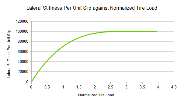
A good starting value for latStiffX is somewhere between 2 and 3. A good starting value for mLatStiffY is around 100000.
camberStiff:
Camber stiffness is analogous to the longitudinal and lateral stiffness, except that it describes the camber thrust force arising per unit camber angle (in radians). The independent camber force is computed as the camber angle multiplied by the camber stiffness:
camberTireForce = camberStiff * camberAngle;
frictionVsSlip:
These six values describe a graph of friction as a function of longitudinal slip. Vehicle tires have a complicated response to longitudinal slip. This graph attempts to approximate this relationship.
Typically, tires have a linear response at small slips. This means that when the tire is only slightly slipping it is able to generate a response force that grows as the slip increases. At greater values of slip, the force can actually start to decrease from the peak value that occurs at the optimum slip. Beyond the optimum slip the tire eventually starts behaving less and less efficiently and hits a plateau of inefficiency.
The friction value for the combination of surface type and tire type is stored in the value PxVehicleRoadGeometryState::friction. The graph of friction versus longitudinal slip is used as a correction. In particular, a final friction value is computed from the product of PxVehicleRoadGeometryState::friction and the value taken from the friction vs slip graph. The tire model then responds to the final friction value.
The first two values describe the friction at zero tire slip: frictionVsSlip[0][0] = 0, and frictionVsSlip[0][1] = friction at zero slip.
The next two values describe the optimum slip and the friction at the optimum slip: frictionVsSlip[1][0] = optimum slip, frictionVsSlip[1][1] = friction at optimum slip.
The last two values describe the slip at which the plateau of inefficiency begins and the value of the friction available at the plateau of inefficiency: frictionVsSlip[2][0] = slip at the start of the plateau of inefficiency, frictionVsSlip[2][1] = the friction available at the plateau of inefficiency.
In the graph below the following values have been used:
frictionVsSlip[0][0] = 0.0
frictionVsSlip[0][1] = 0.4
frictionVsSlip[1][0] = 0.5
frictionVsSlip[1][1] = 1.0
frictionVsSlip[2][0] = 0.75
frictionVsSlip[2][1] = 0.60
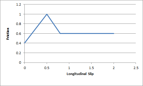
The friction values described here are used to scale the friction of the ground surface. This means they should be in range (0,1) but this is not a strict requirement. Typically, the friction from the graph would be close to 1.0 in order to provide a small correction to the ground surface friction.
A good starting point for this is a flat graph of friction vs slip with these values:
frictionVsSlip[0][0]=0.0
frictionVsSlip[0][1]=1.0
frictionVsSlip[1][0]=0.5
frictionVsSlip[1][1]=1.0
frictionVsSlip[2][0]=1.0
frictionVsSlip[2][1]=1.0
loadFilter:
This is for very fine control of the handling, and corrects numerical issues inherent in simulations at large timesteps.
At large simulation timesteps the amplitude of motion of the suspension springs is larger than it would be in real-life. This is unfortunately unavoidable. On a bumpy surface this could mean that the simulation lifts the car further from the ground than would really happen. This could be quickly followed by the spring being more compressed than would be experienced with a real vehicle. A consequence of this oscillation is that the load on the tire is more variable than expected, and the available tire forces have more variability than expected. This filter aims to correct this numerical problem by smoothing the tire load with the aim of making the handling smoother and more predictable.
A key concept is that of normalized tire loads. A normalized tire load is just the actual load divided by the load experienced when the vehicle is in its rest configuration. If a tire experiences more load than it does at rest then it has a normalized tire load greater than 1.0. Similarly, if a tire has less load than it does at rest then it has a normalized tire load less than 1.0. At rest, all tires obviously have a normalized tire load of exactly 1.0. The normalized tire load can never be less than zero.
The values here describe points on a 2d graph that generates filtered tire loads from raw tire loads. The x-axis of the graph is “normalized tire load”, while the y-axis of the graph is “filtered normalized tire load”. The values loadFilter[0][0] and loadFilter[1][0] are respectively the x-coordinates of the beginnng and end of the linear portion of the graph. The values loadFilter[0][1] and loadFilter[1][1] are respectively the y-coordinates of the beginning and end of the linear portion of the graph.
Normalized loads less than loadFilter[0][0] produce a filtered normalized load of loadFilter[0][1]. Normalized loads greater than loadFilter[1][0] produce a filtered normalized load of loadFilter[1][1]. Loads in-between loadFilter[0][0] and loadFilter[1][0] produce a filtered normalized load in-between loadFilter[1][0] and loadFilter[1][1], as computed by direct interpolation.
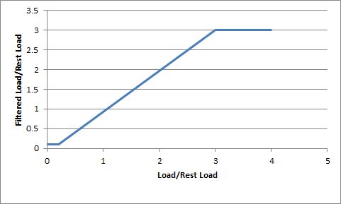
Choosing loadFilter[1][0] and loadFilter[1][1] limits the maximum load that will ever be used in the simulation. On the other hand, choosing loadFilter[0][0]>0 and/or loadFilter[0][1]>0 allows the tire to potentially generate a non-zero tire force even when the tire is just touching the ground at maximum droop.
The filtered load can be made identical to the computed tire load by setting:
loadFilter[0][0]=loadFilter[0][1]=0
loadFilter[1][0]=loadFilter[1][1]=1000.
Note
Tires may only generate forces if the tire is touching the ground: if the tire cannot be placed on the ground then the tire force is always of zero magnitude. A tire touching the ground at maximum suspension droop, on the other hand, has zero measured load because the spring generates zero force at maximum droop. By editing loadFilter it is possible to generate tire forces even when there is very little load actually acting on the tire.
PxVehicleRigidBodyParams
This is used by direct and engine drive models to specify the physics of the vehicle’s rigid body representation.
moi:
The moment of inertia of the rigid body is an extremely important parameter when editing vehicles because it affects the turning and rolling of the vehicle.
A good starting point for the moment of inertia of the rigid body is to work out the moment of inertia of the cuboid that bounds the chassis geometry. If the bounding cuboid is W wide, H high, and L long then the moment of inertia for a vehicle of mass M is:
((L*L+H*H)*M/12, (W*W+L*L)*M/12, (H*H+W*W)*M/12)However, this is only a rough guide. Tweaking each value will modify the motion around the corresponding axis, with higher values making it harder to induce rotational speed from tire and suspension forces.
Providing unphysical values for the moment of inertia will result in either very sluggish behavior or extremely twitchy and perhaps even unstable behavior. The moment of inertia must at least approximately reflect the length scales of the suspension and tire force application points.
This parameter should be viewed as one of the first go-to editable values.
mass:
A typical car might have a mass of around 1500kg.
PxVehicleDirectDriveThrottleCommandResponseParams
This is used by the direct drive model to specify the per wheel drive torque response to a throttle command.
maxResponse:
This is the maximum achievable drive torque that corresponds to the throttle pedal maximally applied.
wheelResponseMultipliers:
This is the per wheel response as a multiplier typically in range [-1,1]. A negative multiplier indicates that the wheel is negatively geared, while a positive mutiplier indicates that the wheel is positively geared. Front wheel drive may be implemented by applying 1.0 to the front wheels and 0.0 to the rear wheels. Conversely, applying 0.0 to the front and 1.0 to the rear implements rear wheel drive.
PxVehicleEngineParams
This is used by engine drive models to specify the drive torque response of the engine to a throttle command.
moi:
This is the moment of inertia of the engine around the axis of rotation. Larger values make it harder to accelerate the engine, while lower values make it easier to accelerate the engine. A starting value of 1.0 is a good choice.
peakTorque:
This is the maximum torque that is ever available from the engine. A starting value might be around 600, if expressed in Newton Metres.
torqueCurve:
This is a graph of peak torque versus engine rotational speed. Cars typically have a range of engine speeds that produce good drive torques, and other ranges of engine speed that produce poor torques. A skilled driver will make good use of the gears to ensure that the car remains in the “good” range where the engine is most responsive. Tuning this graph can have profound effects on gameplay.
The x-axis of the curve is the normalized engine speed; that is, the engine speed divided by the maximum engine speed. The y-axis of the curve is a multiplier in range (0,1) that is used to scale the peak torque.
idleOmega:
This is the lowest rotational speed of the engine, expressed in radians per second.
maxOmega:
This is the maximum rotational speed of the engine, expressed in radians per second.
dampingRateFullThrottle:
dampingRateZeroThrottleClutchEngaged:
dampingRateZeroThrottleClutchDisengaged:
These three values are used to compute the damping rate that is applied to the engine. If the clutch is engaged then the damping rate is an interpolation between dampingRateFullThrottle and dampingRateZeroThrottleClutchEngaged, where the interpolation is governed by the acceleration control value generated by the gamepad or keyboard. At full throttle dampingRateFullThrottle is applied, while dampingRateZeroThrottleClutchEngaged is applied at zero throttle. In neutral gear the damping rate is an interpolation between dampingRateFullThrottle and dampingRateZeroThrottleClutchDisengaged.
The three values allow a range of effects to be generated: good acceleration that isn’t hampered by strong damping forces, tunable damping forces when temporarily in neutral gear during a gear change, and strong damping forces that will bring the vehicle quickly to rest when it is no longer being driven by the player.
Typical values in range (0.25,3). The simulation can become unstable with damping rates of 0.
PxVehicleGearboxParams
This is used by engine drive models to specify the gearing ratio of each gear of the vehicle and the number of gears.
neutralGear:
This is the index of the neutral gear. All gears with higher gear index are considered to be forward gears and all gears with lower gear index are considered to be reverse gears. A vehicle with a single revese gear would have a neutral gear with index 1.
nbRatios:
This is the number of the gears of the vehicle, including all reverse gears and neutral gear. A standard car with 5 forward gears would, therefore, have a value of 7 after accounting for reverse and neutral.
ratios:
Each gear requires a gearing ratio. Higher gear ratios result in more torque but lower top speed in that gear. Typically, the higher the gear, the lower the gear ratio. Neutral gear must always be given a value of 0, while reverse gear must have a negative gear ratio. Typical values might be 4 for first gear and 1.1 for fifth gear.
finalRatio:
The gear ratio used in the simulator is the gear ratio of the current gear multiplied by the final ratio. The final ratio is a quick and rough way of changing the gearing of a car without having to edit each individual entry. Further, quoted gearing values from manufacturers typically mention ratios for each gear along with a final ratio. A typical value might be around 4.
switchTime:
The switch time describes how long it takes (in seconds) for a gear change to be completed. It is impossible to change gear immediately in a real car. Manual gears, for example, require neutral to be engaged for a short time before engaging the desired target gear. While the gear change is being completed the car will be in neutral. A good trick might be to penalize players that use an automatic gear box by increasing the gear switch time.
If the autobox is enabled it is a good idea to set this value significantly lower than PxVehicleAutoboxParams::latency. If the autobox latency is smaller than the gear switch time then the autobox might decide to initiate a downwards gear change immediately after an upward gear shift has been completed. This situation can leave the car cycling between neutral and first gear with very short interludes in 2nd gear.
PxVehicleAutoboxParams
This is used by engine drive models to specify the operation of the automatic gearbox.
The autobox initiates gear changes up or down based on the rotation speed of the engine. If the engine is rotating faster than a threshold value stored in PxVehicleAutoBoxData then a gear increment will be initiated. On the other hand, if the engine is rotating slower than a threshold value then the autobox will initiate a gear decrement. The autobox only initiates gear changes upward or downwards a single gear at a time.
It is worth noting that if the autobox initiates a gear change then the accelerator pedal is automatically disconnected from the engine for the entire duration of the gear change. Manual gear changes are not subject to this limitation. This is in keeping with typical real-world autobox behavior. The idea behind this is to stop the engine wildly accelerating during the neutral phase of the gear change, thereby avoiding damaging clutch slip when the clutch re-engages at the end of the gear change.
The autobox will not try to initiate a gear change while an automatic or manual gear change is still active.
The autobox can be readily enabled and disabled by setting PxVehicleEngineDriveTransmissionCommandState::targetGear to either an indexed gear or to the value PxVehicleEngineDriveTransmissionCommandState::eAUTOMATIC_GEAR.
PxReal upRatios[PxVehicleAutoboxParams::eMAX_NB_GEARS]:
The autobox will initiate a gear increment if the ratio of the engine rotation speed to the maximum allowed engine rotation speed:
PxVehicleEngineState::rotationSpeed() / PxVehicleEngineParams::maxOmegais greater than the value stored in upRatios[PxVehicleGearboxState::currentGear]
PxReal downRatios[PxVehicleAutoboxParams::eMAX_NB_GEARS]:
The autobox will initiate a gear decrement if the ratio of the engine rotation speed to the maximum allowed engine rotation speed:
PxVehicleEngineState::rotationSpeed() / PxVehicleEngineParams::maxOmegais less than the value stored in downRatios[PxVehicleGearboxState::currentGear]
latency:
After the autobox has initiated a gear change it will not attempt to initiate another gear change until the latency time has passed. It is a good idea to set this value significantly higher than PxVehicleGearboxParams::switchTime. If the latency is smaller than the gear switch time then the autobox might decide to initiate a downwards gear change immediately after an upward gear shift has been completed. This situation can leave the car cycling between neutral and first gear with very short interludes in 2nd gear.
PxVehicleClutchCommandResponseParams
This is used by engine drive models to specify the clutch strength response to a clutch command.
maxResponse:
This describes the maximum strength of the coupling between the wheels and engine. The instantaneous strength is the product of maxResponse and (1.0f -PxVehicleEngineDriveTransmissionCommandState::clutch).
Smaller values will result in more clutch slip, especially after changing gear or stamping on the accelerator. Higher values will result in reduced clutch slip, and more engine torque delivered to the wheels.
This value is to be edited only for very fine tweaking of the vehicle. Some clutch slip can be attributed to the numerical issues in the simulation at large timesteps, while some is a natural consequence of driving the car in an overly aggressive manner. A value of 10 is a good starting point.
PxVehicleClutchParams
This is used by engine drive models to specify the computational method used to resolve the coupling between engine and wheels.
PxVehicleClutchParams specifies the algorithm employed to resolve the differential equations that couple engine and wheels. If the wheel count is large, the computation corresponding to PxVehicleClutchAccuracyMode::eBEST_POSSIBLE becomes expensive and it could be beneficial to use PxVehicleClutchAccuracyMode::eESTIMATE instead. If estimation mode is selected then the parameter PxVehicleClutchAccuracyMode::estimateIterations may be used to control the trade-off of computational effort and performance.
As a guide, it is recommended to use PxVehicleClutchAccuracyMode::eBEST_POSSIBLE for a vehicle with four wheels connected to the differential. At the other end of the spectrum, a truck with 20 wheels connected to the drivetrain will require PxVehicleClutchAccuracyMode::eESTIMATE.
PxVehicleMultiWheelDriveDifferentialParams
This is used by engine drive models to specify a differential that distributes drive torque to each wheel using a constant multiplier. It also describes the contribution that each wheel makes to the averaged rotational speed of the wheel-side clutch plate.
torqueRatios:
For a four-wheeled vehicle, front(rear) wheel drive may be implemented by applying 0.5 to both front(rear) wheels. Alternatively, drive torque may be deliverd to all wheels of a vehicle. For a four-wheeled vehicle this would require a value of 0.25 to be applied to both front and both rear wheels. The sum of all entries in the torqueRatios must add up to 1.0.
aveWheelSpeedRatios:
The clutch is modelled as two spinning plates with one plate connected to the engine and the other connected to the wheels. The torque delivered to the wheels is proportional to the rotational speed difference between the two plates. The rotational speed of wheel-side clutch plate is computed as a weighted average with the weights governed by the array aveWheelSpeedRatios. A good starting point is to set each entry in aveWheelSpeedRatios to be the same as the equivalent entry in the torqueRatios array.
PxVehicleFourWheelDriveDifferentialParams
This is used by engine drive models to specify a differential that distributes torques to wheels with the caveat that specified pairs of wheels obey a rule that their rotational speed ratio never exceeds a configurable differential bias.
PxVehicleFourWheelDriveDifferentialParams performs the same role as PxVehicleMultiWheelDriveDifferentialParams but with the option to turn it into a limited slip differential. The limited slip differential imposes limits on the ratio of wheel rotational speed when considering pairs of wheels. The class PxVehicleFourWheelDriveDifferentialParams introduces the vocabulary of front wheels and rear wheels. A maximum ratio may be specified for a pair of wheels specified as front wheels. Equally, a maximum ratio may be specified for a pair of wheels specified as rear wheels. Finally, a maximum ratio may be specified for the front wheel pair relative to the rear wheel pair.
In the absence of any breach of a slip limit, drive torque is distributed to the wheels as specified in the torqueRatios array. Beyond the slip limit, torque is diverted from one wheel of a limited slip pair to the other.
frontWheelIds[2]:
The array frontWheelIds specifies the two wheels considered by the limited slip differential as front wheels.
rearWheelIds[2]:
The array rearWheelIds specifies the two wheels considered by the limited slip differential as rear wheels.
frontBias:
rearBias:
centerBias:
The effect of the limited slip differential is to impose a maximum ratio of wheel rotational speed between pairs of wheel. The parameter frontBias is the maximum allowed for the front wheels, while rearBias is the maximum allowed for the rear wheels. The parameter centerBias is the ratio for the front wheel pair relative to the rear wheel pair. A value of 1.3 is a good starting point for any bias.
frontTarget:
rearTarget:
centerTarget:
If any wheel pair exceeds its bias, the differential will seek to resolve the discrepancy between the current ratio and the specified bias. A problem may arise if the limited slip only just fails to resolve the discrepancy. If this happens, the bias will be breached at the next simulation step and perhaps the next and so on. To avoid this, the differential sets a target rotational speed ratio that is just less than the complementary bias. When the target is much less than the bias it is likely that an oscillation will result with the amplitude of oscillation being proportional to the difference between target and bias. The ideal outcome is a target that does not result in obvious oscillation but also resolves the bias breach without getting stuck in a phase of continual resolution. A value of 1.29 is a good starting point, assuming a bias of 1.3.
rate:
The rate parameter determins the time taken to resolve any discrepancy that arises between the rotational speed ratio of any pair and the bias for that pair.
PxVehicleTankDriveDifferentialParams
This is used by engine drive models to implement a tank differential. The tank differential is designed to deliver torque to the wheels on each tank track in such a way that wheels sharing a tank also share a rotational speed.
The only difference between PxVehicleTankDriveDifferentialParams and PxVehicleMultiwheelDriveDifferentialParams is that PxVehicleTankDriveDifferentialParams requires the wheels on each tank track to be configured. Multiple tank tracks are allowed and each may be linked to a left or right thrust lever.
A wheel on a tank may be added to a track or it may be modelled as a normal wheel that is either connected to the differential or not. Any wheel on a tank may be steered. It is, however, unusual to steer any wheel on a tank track because tank steering is typically achieved by asymmetrically distributing drive and brake torque.
Troubleshooting
This Section introduces common solutions to common problems with vehicle tuning.
Jittery Vehicles
Does the length scale of PxTolerancesScale applied to the PxScene match the length scale of the vehicle (eg. 100 if centimeters are used)? Make sure they match be either updating PxTolerancesScale::length or invoking the relevant transformAndScale() functions for all vehicle parameters.
Is the natural frequency of the spring too high/timestep of simulation too small for reliable simulation? See Section PxVehicleSuspensionForceParams for more details and update the natural frequency or timestep accordingly. Remember that substeps may be applied to the stiffest parts of the vehicle’s update, as discussed in Section Component Sequences.
Is PxVehicleSuspensionParams::suspensionTravelDist set to a value that allows suspension motion?
The Engine Rotation Refuses To Spin Quickly
Are the tires resisting the engine motion through excessive friction forces? Place the car very high above the ground and accelerate the engine to see if the engine and wheels start to spin round.
Do the engine’s moment of inertia, peak torque and damping rates reflect the length scale? Note the documented SI units of each variable and recompute the values as appropriate.
Is the moment of inertia too large? A value of 1 or its equivalent in the relevant length scale is a good estimate for testing purposes.
Is the peak torque too small to drive the engine? Scale the default peak torque value with the mass of the vehicle with the knowledge that the default value will drive a standard car of around 1500kg.
Does the torque curve contain sensible values? Try a flat curve with each data point having a y-value of 1.0.
Is the maximum engine angular speed a realistic value? Consult any available manufacturer data for typical values or revert to the default value for testing purposes.
Are any of the damping rates too high? Reduce the damping rates and test.
The Engine Spins But the Wheels Refuse To Spin
Is the vehicle in neutral gear? Connect the engine to the wheels by setting the gear as appropriate and disabling the autobox.
Does the differential deliver drive torque to the wheels? Make sure that the differential is properly configured.
Is the brake or handbrake engaged? Ensure that the brake and handbrake are both zero.
Do the wheels’ moment of inertia and damping rates reflect the length scale? Note the documented SI units of each variable and recompute the values as appropriate.
Are the wheels’ moments of inertia too high? Recompute the wheels’ moments of inertia.
Are the wheels’ damping rates too high? Reduce the wheels’ damping rates.
Are the tires resisting the engine motion through excessive friction forces? Place the car very high above the ground and accelerate the engine to see if the engine and wheels start to spin round.
The Wheels Are Spinning But The Vehicle Does Not Move Forwards
Is the filtering configured so that the vehicle is supported only by suspension forces? Check the filtering configuration for shapes attached to the vehicle’s rigid body actor, search for contacts involving shapes attached to the vehicle’s actor using PVD.
Is sufficient friction being delivered to the tire?
Do the suspension forces (and the loads on the tires) reflect the mass of the rigid body actor? A 4-wheeled vehicle should generate suspension forces of approximately actorMass*gravity/4. Adjust the sprung masses of the vehicle suspensions to ensure that the driven wheels experience significant tire load.
Do the tires generate significant longitudinal tire forces? Check that the longitudinal slip of the tire is non-zero and approaches 1.0 when the wheels are spinning quickly without forward motion.
Is the tire longitudinal stiffness too small? Adjust the longitudinal stiffness back to the default value and test.
Is the mass of the vehicle’s rigid body actor too large to be driven by the engine peak torque? Test that the mass of the actor is a sensible value and set accordingly.
Is the rigid body actor in a PhysX scene and is the scene being updated? Ensure that the actor is not asleep and participates in the scene update.
The Vehicle Does Not Steer/Turn
Is the moment of inertia of the vehicle too large so that it resists turning motion? Check that the moment of inertia of the vehicle’s rigid body actor is a sensible value. Use the moment of inertia of a box with width/height/length of the vehicle as a starting guess for the moment of inertia of the actor.
Are the steer wheels receiving a steer angle? If the steer angle is zero or smaller than expected check that a steer angle is being passed to the vehicle and that the maximum steer angles of the steer wheels are sensible values.
Do the steer wheels have a sensible lateral slip angle?
Is the lateral stiffness of the tire configured properly?
The Acceleration Feels Sluggish
Are the damping rates of the engine and wheels too large? Reduce the engine damping rate, then the wheel damping rates and retest each time.
Is the vehicle stuck in the same gear all the time? Disable the autobox and change gears manually to test if the autobox is failing to switch gear. Check the autobox settings to make sure that it will automatically increase the gear at sensible engine rotation speeds.
Is the engine powerful enough to quickly accelerate the car? Increase the peak torque of the engine.
Do the wheels have high moments of inertia that prevent significant longitudinal slips developing? Reduce the moments of inertia of the wheels.
The Vehicle Does Not Slow Down When Not Accelerating
Are the wheel and engine damping rates too small? First increase the engine damping rate, then the wheel damping rates and retest each time.
Does the vehicle’s rigid body actor have a velocity damping value? Increase as appropriate.
The Vehicle Turns Too Quickly/Too Slowly
Does the moment of inertia of the rigid body actor need tweaking? Adjust the component of the moment of inertia that corresponds to motion about the up vector. Increasing the moment of inertia will slow the turn rate, decreasing the moment of inertia will increase the turn rate.
The Wheels Spin Too Much Under Acceleration
Is the accelerator pedal value increasing too rapidly from 0 to 1? Slow down the rate of increase of the accelerator pedal value by filtering the controller or keyboard. Remember that aggressively pressing the accelerator pedal on a powerful car ought to lead to wheel spin.
Are the wheel moments of inertia too low? Increase the wheel moments of inertia.
The Wheels Spin Too Much When Cornering
Does the vehicle have a limited slip differential? If applicable set the differential type to limited slip and adjust the differential biases accordingly.
The Vehicle Never Goes Beyond First Gear
Does the vehicle cycle between first gear and neutral? If the autobox is enabled then the problem is probably that the latency of the autobox is shorter than the time spent performing a gear change. The autobox latency controls the minimum time spent in-between automated gear changes. After an automated gear change is initiated the autobox will not make another gear change decision until the latency time has passed. During a gear change the vehicle enters neutral gear and the accelerator pedal is uncoupled from the engine, meaning that the engine will slow down during the gear change. When the vehicle enters the target gear at the end of the gear change the autobox might decide immediately that the engine is too slow for the target gear and immediately initiate a downwards gear change. This will immediately put the car back in neutral, meaning that the car spends a very long time in neutral and never reaches its target gear. This will not happen if the autobox latency is set significantly larger than the gear switch time.
The Vehicle Under-steers Then Over-steers
Is the vehicle on a bumpy surface? Edit the values in PxVehicleTireForceParams::loadFilter so that the filtered normalized tire load has a flatter response to suspension compression.
The Vehicle Slows Down Unnaturally
Does the vehicle not slow down smoothly to rest? Take a look at the longitudinal slip values to see if they are oscillating between positive and negative. If there is a strong oscillation then two options are available that can be used separately or in conjunction with each other. The first option is to use substepping to force more vehicle update sub-steps as the forward speed of the vehicle approaches zero. The second option is to use PxVehicleTireSlipParams::minPassiveLongSlipDenominator to ensure that the denominator of the longitudinal slip never falls below a specified value.
The Vehicle Climbs Too Steep Slopes
Are the front wheels slipping badly? Modify PxVehicleTireForceParams::frictionVsSlip to reduce the available friction for slipping wheels.
References
Anti-roll Bar
Tire Modeling
The default tire model employed by PhysX vehicles is discussed in Appendix H of the CarSimEd documentation:
A tire model commonly used in engineering simulation is the Pacejka tire model: