

Non-Visual Sensors#
Non-visual sensors simulate lidar, radar and ultrasonic measurements by tracing rays through the scene. They produce point clouds, radar detections or echo envelopes. Surface materials affect the strength and timing of returns; wave-propagation models also account for paths with multiple surface interactions.
Sensor models#
ovrtx provides five non-visual sensor models. The sensor prim type and applied API schema select the model. Each model has its own attributes and output channels; see Sensor Configuration for the shared setup.
Model |
Simulation |
Output |
|---|---|---|
Rotary or solid-state scanning lidar, using scheduled emitter firings and geometric ray intersections. |
PointCloud: lidar returns. |
|
Pulsed time-of-flight lidar with wave propagation, surface interactions and detector response. |
PointCloud: returns derived from the received signal and the selected return-processing mode. |
|
Radio-wave propagation into a detection matrix, including multiple bounces, material response and transmit/receive antenna patterns. |
PointCloud: detections with position, radial velocity and radar cross section (RCS). |
|
Ultrasonic pulses. Each firing event selects a transmitting mount and a group of receiving mounts. |
SignalWays: echo amplitude over time for each receiving mount and channel ID. |
|
Scalar electromagnetic or mechanical propagation with independently authored transmitter, receiver and ray patterns. |
Contributions: raw paths, scalar transport power and validity, before detector processing. |
The two lidar models both use an OmniLidar prim. Apply
OmniSensorGenericLidarCoreAPI for geometric scanning, or
OmniSensorGenericLidarWpmAPI when pulse propagation and detector response
matter. Their attributes and output channels differ; the
Lidar wpm overview compares them.
Radar uses OmniRadar with OmniSensorGenericRadarWpmDmatAPI. Its default
carrier frequency is approximately 77 GHz. One radar can have multiple scan
configurations, such as near and far scans; see the
radar overview.
Acoustic sensors use OmniAcoustic with OmniSensorGenericAcousticWpmAPI.
Their repeating firing sequence determines which mounts transmit and listen.
The Generic wpm model uses OmniGeneralSensor with
OmniSensorGenericWpmAPI. Choose it when your application consumes raw path
contributions and supplies its own detector processing.
Configuration and outputs#
Bind materials with non-visual labels to describe surface response. The labels are separate from visual shading; some models can also use visual material inputs. See Non-Visual Sensor Materials.
Motion BVH accounts for sensor and geometry motion within a scan. Use AUTO
or ENABLE for lidar and radar motion effects and for acoustic simulation. See Motion BVH
for renderer configuration and hardware requirements.
Each model returns a composite output containing named tensors and parameters. See Sensor Outputs for mapping and reading it. Lidar and radar positions default to spherical coordinates: azimuth and elevation in degrees, and range in meters. Cartesian output uses x, y and z in meters. Acoustic output contains signal samples rather than positions. Generic wpm output uses a dense contribution layout with explicit validity. The linked Outputs pages above define each model’s channels and coordinate options.
Examples#
Start with Your First Lidar Sensor for a Lidar core setup. The runnable lidar example is available in Python and C; the Lidar core tutorials configure three physical devices. For Lidar wpm, see the rotary example scene in Configure a Firing Pattern.
The radar example is available in Python and C.
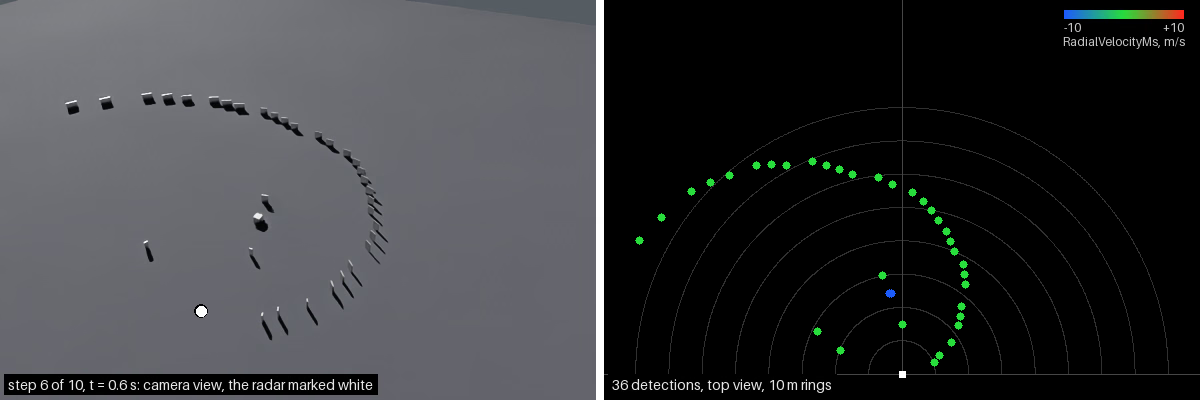
Radar example: a steel cube moves among steel panels over asphalt. Left: camera view. Right: detections colored by radial velocity. Blue approaches the sensor, green is near zero, and red recedes.#
The Python acoustic example shows an ultrasonic echo from a wall. There is no corresponding C example.
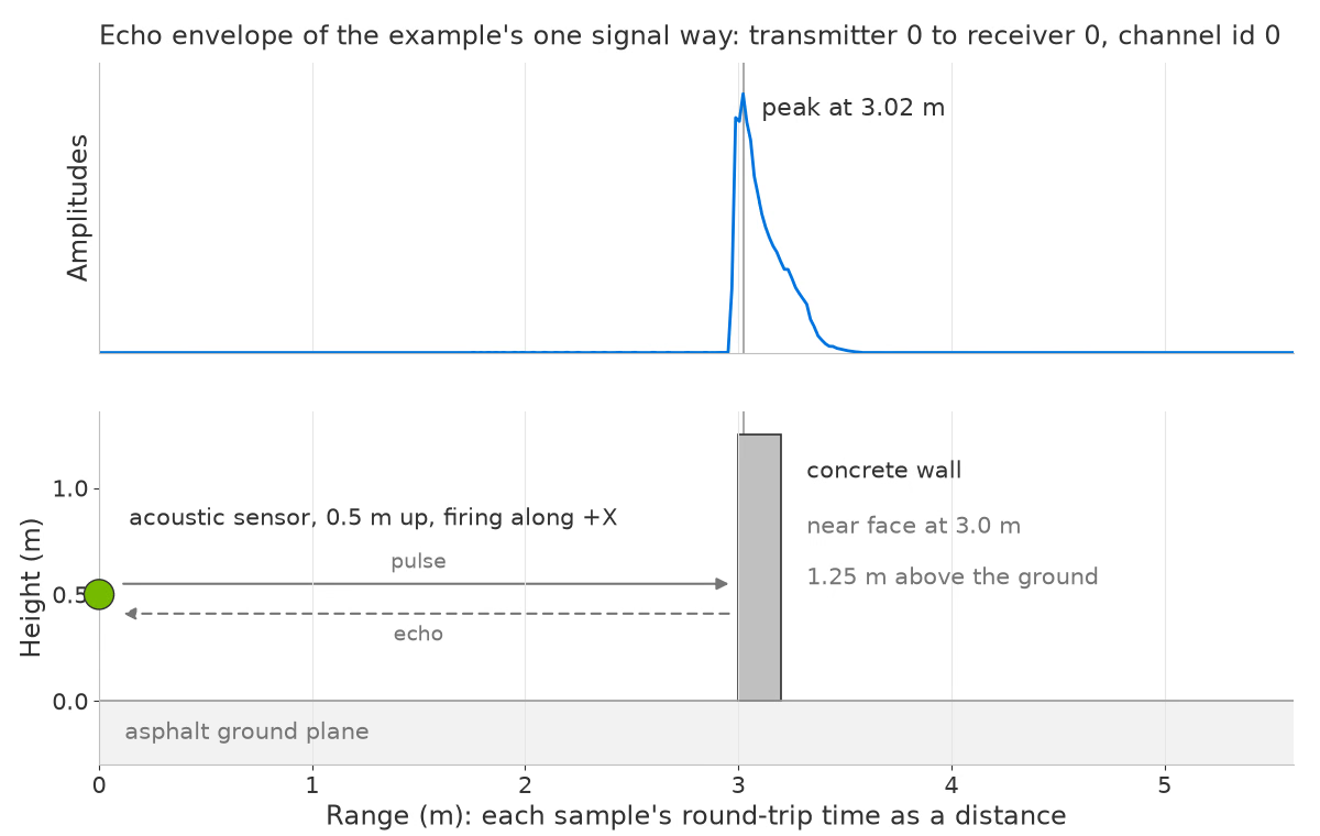
Acoustic example: a sensor 0.5 m above asphalt faces a concrete wall 3 m ahead. The echo peak aligns with the wall. The plot converts round-trip time to range and shows one signal way.#
The Generic wpm recipes run in Python and C. They demonstrate depth sampling, full-circle scans, finite beams, independent receivers and mechanical propagation.