Outputs

The Radar generic wpmDmat model delivers one PointCloud composite output per requesting RenderVar. It contains per-detection tensors, two automatically included tensors and CPU-resident parameters describing the frame and scan. See USD Attributes for output controls and Sensor Outputs for mapping and container access.

Each entry represents a detection accepted by processing, rather than a ray hit. There is no per-emitter, per-echo or per-surface information. Each published radar frame contains one scan, which may have zero detections.

An object can produce multiple detections or none. Multipath can produce ghost detections whose ranges follow the propagation path. RadialVelocityMs measures direct-path line-of-sight motion or, for multipath returns, motion projected along the propagation segments. See Radar generic wpmDmat model.

Requesting the output

A radar scene needs a RenderProduct whose camera relationship names the OmniRadar prim and whose orderedVars names a RenderVar with sourceName = "PointCloud"; the RenderVar’s channels attribute lists the tensors to produce. Output Configuration explains RenderProducts, RenderVars and the channels attribute in general. The example below requests coordinates, radar cross section and radial velocity. Omit RCS from channels when you do not need it.

USDA

#usda 1.0
    def "Render"
    {
        def "Products"
        {
            def RenderProduct "RadarProduct"
            {
                rel camera = </World/Radar>
                rel orderedVars = [<../../Vars/PointCloud>]
            }
        }

        def "Vars"
        {
            def RenderVar "PointCloud"
            {
                uniform string sourceName = "PointCloud"
                token[] channels = [
                    "Coordinates",
                    "Counts",
                    "RCS",
                    "RadialVelocityMs"
                ]
            }
        }
    }

USD Python

from pxr import Gf, Sdf

world = stage.DefinePrim("/World", "Xform")

render = stage.DefinePrim("/World/Render", "")

products = stage.DefinePrim("/World/Render/Products", "")

radar_product = stage.DefinePrim("/World/Render/Products/RadarProduct", "RenderProduct")
radar_product.CreateRelationship("camera", custom=False).SetTargets(["/World/Radar"])
radar_product.CreateRelationship("orderedVars", custom=False).SetTargets(
    ["/World/Render/Vars/PointCloud"]
)

vars = stage.DefinePrim("/World/Render/Vars", "")

point_cloud = stage.DefinePrim("/World/Render/Vars/PointCloud", "RenderVar")
point_cloud.CreateAttribute(
    "sourceName", Sdf.ValueTypeNames.String, custom=False, variability=Sdf.VariabilityUniform
).Set("PointCloud")
point_cloud.CreateAttribute("channels", Sdf.ValueTypeNames.TokenArray, custom=False).Set(
    ["Coordinates", "Counts", "RCS", "RadialVelocityMs"]
)

The names you can list are Coordinates, RCS, TimeOffsetNs, RadialVelocityMs and Flags. Counts and Flags are added whether or not you list them, so the Counts entry the example scenes author is permitted but not required. How the list is read, what an unknown name does and several PointCloud RenderVars on one product are on channels.

Channels

The table lists every channel a radar PointCloud can carry. Nmax is the capacity of the per-detection tensors, the number of entries each of them is allocated for. The model publishes it beside the channels as the maxPoints param, and for this model it is the fixed detection cap described below. The entries a frame delivered are the first Counts[0] of them.

Channel	Type	Shape	Unit	Meaning
Counts	int32	[1]	detections	Number of entries delivered this frame. Bounds every per-detection tensor. Always published.
Flags	uint8	[Nmax]	unitless	Per-detection status bits. The VALID bit is 0x40; this model sets no other bit. Always published.
Coordinates	float32	[3, Nmax]	m, or deg / deg / m	Position of the detection in the configured representation and frame, packed component-first. Cartesian rows are x, y and z in meters; spherical rows, the default, are azimuth and elevation in degrees followed by range in meters.
RCS	float32	[Nmax]	dBsm	Radar cross section: a logarithmic measure, in decibel square meters, of how detectable the target is. The value depends on the scan’s RCS calibration attributes and scene. Compare the range of values across a frame when evaluating response. It is clamped to [-60, 60] dBsm; detections below the scan’s minimum accepted RCS are dropped (rcsTuningCoefficients).
RadialVelocityMs	float32	[Nmax]	m/s	Doppler radial velocity along the line of sight. Signed; approaching detections are negative.
TimeOffsetNs	int32	[Nmax]	ns	Time offset of the detection within the scan. 0 for every detection, because the model simulates a scan at one instant.

RCS, dBsm and the other radar terms are defined in the glossary; the RCS calibration attributes, rcsTuningCoefficients among them, are on USD Attributes. The subsections below say how to read each channel.

Counts, Flags and the detection cap

Counts[0] gives the number of delivered entries. Read only slots [0, Counts[0]); the tensor length is allocated capacity. See reading a variable-size output.

• A scan produced detections: Counts[0] is the detection count.

• A scan produced no detections: Counts[0] is 0 and the output still carries the scan’s parameters and acquisition timestamp.

• No scan fired: no radar frame is published. This occurs when the pending scan’s acquisition time falls outside the step’s time window, commonly when simulation steps are shorter than the radar’s scan period.

A scan can fire at time zero, so timestampNs = 0 is a valid acquisition timestamp. See stepping and delivery for aligning steps with scans, and Sensor Scheduling for sensors running at different rates.

Empty scans

A scan with no detections publishes Counts[0] = 0. Its scan parameters, including scanIdx, cycleCnt and timestampNs, still describe that acquisition. Per-detection tensors retain their allocated capacity, but have no delivered entries to read. Use Counts[0] to recognize an empty scan; no RCS channel is needed for this check.

Validity flags

Every delivered detection has the VALID bit set. No other flag bits are set. Radar has no includeInvalidPoints option and does not include invalid slots within [0, Counts[0]).

Test validity with Flags[i] & 0x40, as the radar examples do. Avoid an exact comparison with 0x40 so the reader also works with models that set additional bits. See validity flags.

Detection limit

Each scan can report up to 2500 detections. Additional detections are dropped without a saturation indicator. maxPoints and the per-detection tensor shapes report this fixed capacity; Counts[0] bounds the entries to read. See allocated capacity.

Coordinate controls

omni:sensor:WpmDmat:elementsCoordsType selects the coordinate representation; outputFrameOfReference selects the reference frame, and customFrameOfReferenceTrafo supplies its pose when set to CUSTOM. See coordinate controls for tokens, units and defaults. The radar ignores the lidar’s omni:sensor:Core:* attributes (namespaces).

The SENSOR frame uses ISO 8855 axes. Read coordsType and frameOfReference from each output to identify the active settings, particularly after a runtime update.

Coordinates is packed component-first: all the x values, then all the y, then all the z (or all the azimuths, all the elevations, then all the ranges), with the capacity as the step between components, not the delivered count. The mapped tensor reports this as a shape of [3, Nmax] with strides of [Nmax, 1]. Take the layout from the shape and strides rather than from the channel’s name, because other models pack a channel of the same name differently (Tensor layouts). Both example scenes author CARTESIAN, which is why the Python example plots the delivered columns as x, y, z points without a conversion.

RadialVelocityMs

Approaching detections have negative RadialVelocityMs. To select moving detections in either direction, threshold its absolute value. To distinguish approaching and receding detections, retain the sign. The example’s steel cube moves toward the radar by 1 m per step for ten steps and produces negative values.

A FAST scan folds radial velocity into the interval the frame reports as minVelMps to maxVelMps, so a value inside that interval can belong to a faster target; aliasing and the unambiguous intervals explains the folding and the WAVEFORM case.

Doppler from moving targets needs the renderer’s motion BVH (Motion BVH); the moving-targets how-to says what the model does without it and how to check that the switch was active.

Timestamps

The TimeOffsetNs channel is delivered when requested and holds 0 for every detection, because the model simulates each scan as a single instant. A radar frame therefore carries no per-detection timing. The frame’s own timing is in its params: timestampNs is the scan’s instant, and frameStartTimeStampNs and frameEndTimeStampNs bound the frame’s time window, which can be wider than that instant. Consistent with this, the model has no motion-compensation attribute (Limitations).

The Lidar generic core model defines a channel of the same name differently (the lidar time offset); Model-specific channel semantics gives the rule.

Material identifiers

The radar PointCloud has no MaterialId channel, and no other channel or param names a material: the label a detection came from is not reported. The labels and how to author them are on Non-Visual Sensor Materials.

Params

A radar PointCloud carries CPU-resident parameters: thirteen shared with core lidar and ten radar-specific scan parameters. The table below gives the radar semantics for the shared parameters.

Param	Type	Shape	Value
frameId	uint64	[1]	The model’s frame counter. It never restarts and can skip values between published scans when no acquisition occurs in an intervening time window. It is not a count of delivered scans; use cycleCnt and scanIdx below to follow the scan cycle.
timestampNs	uint64	[1]	The scan’s acquisition time, in nanoseconds: its scan time plus the selected scan’s timeOffsetUsec delay (the frame rate defines both). With omni:sensor:frameRate unset, (0, 1), it equals frameEndTimeStampNs. Zero is valid for a scan acquired at time zero. A scan with no detections still reports its acquisition time.
modality	uint32	[1]	2, radar.
frameOfReference	uint16	[1]	0 sensor, 1 world, 2 custom, as omni:sensor:WpmDmat:outputFrameOfReference selected it.
coordsType	uint32	[1]	0 Cartesian, 1 spherical, as omni:sensor:WpmDmat:elementsCoordsType selected it. Spherical is the default, so an output whose sensor never set the attribute reads 1.
modelToAppTransform	float32	[4, 4]	Transform from the sensor frame to the application frame: a homogeneous transform stored row by row, with a bottom row of 0, 0, 0, 1, whose rotation takes the model’s ISO 8855 axes to the application’s.
frameStartTimeStampNs	uint64	[1]	Start of this frame’s time window, in nanoseconds. The scan’s acquisition time can fall later in this window.
frameStartPosM	float32	[3]	Sensor position at that start, in meters, in the world frame.
frameStartOrientation	float32	[4]	Sensor orientation at that start, as a world-frame unit quaternion ordered x, y, z, w.
frameEndTimeStampNs	uint64	[1]	End of this frame’s time window, in nanoseconds. It does not move when timeOffsetUsec delays the acquisition; timestampNs does.
frameEndPosM	float32	[3]	Sensor position at that end, in meters, in the world frame.
frameEndOrientation	float32	[4]	Sensor orientation at that end, as a world-frame unit quaternion ordered x, y, z, w.
maxPoints	uint32	[1]	The capacity Nmax: the fixed cap of 2500 detections per scan, duplicating the bound already in the per-detection tensors’ shapes.

The shared table on Sensor Outputs lists the full enumerations of modality, frameOfReference and coordsType.

Without the motion BVH the scene does not move within a frame, while the radar itself still does: frameStartPosM, frameStartOrientation, frameEndPosM and frameEndOrientation are its poses at the start and the end of the frame’s time window, the rays fire from its pose at the scan’s acquisition time, frameStartTimeStampNs and frameEndTimeStampNs bound that window, and RadialVelocityMs still reflects the radar’s own movement between frames. The model publishes neither motionCompensationState nor compactionType, the two lidar-only params: it has no motion compensation (Limitations), and it delivers no invalid entries, so there is no compaction to describe.

Scan parameters

The following ten parameters identify the radar model instance, scan configuration and cycle count, and report ambiguity bounds before measurement noise. They accompany every radar PointCloud. See Run More Than One Scan Pattern for scan authoring and cycle verification.

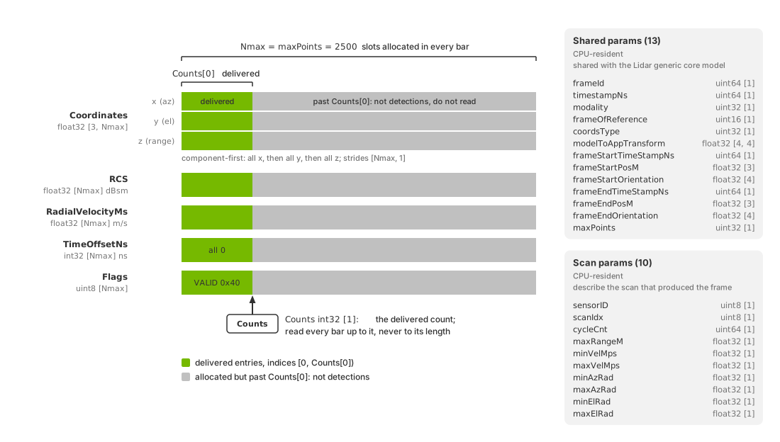
Anatomy of one radar PointCloud output. The per-detection tensors, Coordinates as three component-first rows and RCS, RadialVelocityMs, TimeOffsetNs and Flags as one row each, are allocated for Nmax entries, the maxPoints capacity, and Counts[0] marks how many of them this frame delivered. Beside the tensors sit the CPU params: the thirteen shared with the Lidar generic core model and the ten that describe the scan.

Param	Type	Shape	Value
sensorID	uint8	[1]	A number the process assigns to each radar model instance as it is created, 0 for the first, then 1, 2 and so on, constant for the life of the model. It is not authored and not persistent across runs.
scanIdx	uint8	[1]	Index of the scan configuration this frame used: the position of its instance name in the model’s scan order, counted from 0, so s001 is 0 and s002 is 1. The order and its rules are under Scan instances.
cycleCnt	uint64	[1]	How many times this scan has fired, counted from 0 at its first firing. Firings of other scans and frames that fired no scan do not increase it. The events that restart the velocity sequence restart each scan’s count at 0. It is not frameId, which never restarts.
maxRangeM	float32	[1]	The scan’s maximum unambiguous range, in meters: its maxRangeM attribute as the model resolved it.
minVelMps	float32	[1]	The lower velocity ambiguity bound, in meters per second. In FAST it is the negative of maxVelMps. In WAVEFORM it follows the selected chirp timing and can be asymmetric with nonzero frequency stepping between chirps.
maxVelMps	float32	[1]	The upper velocity ambiguity bound for this frame, in meters per second: the active maxVelMpsSequence entry in FAST, or derived from the selected chirpRepetitionTimeSequence entry, the sensor’s waveLengthMm and the other chirp attributes in WAVEFORM (aliasing). Only the scan that fires advances its sequence (velocity sequence).
minAzRad	float32	[1]	The negative of maxAzRad, in radians.
maxAzRad	float32	[1]	The scan’s azimuth half-angle, its maxAzAngDeg attribute, converted to radians.
minElRad	float32	[1]	The negative of maxElRad, in radians, for every elevMode.
maxElRad	float32	[1]	The scan’s elevation half-angle, its maxElAngDeg attribute, converted to radians.

Compare the output’s scan-limit parameters with the authored values to check the active configuration, including when Counts[0] is zero; configuration verification describes the check. USD Attributes defines maxRangeM, maxVelMpsSequence, the angular half-angles and elevMode.

Angular units

Angular limits and spherical coordinates use different units:

• minAzRad, maxAzRad, minElRad and maxElRad: radians.

• Azimuth and elevation in spherical Coordinates: degrees.

For example, maxAzAngDeg = 75 produces limits of approximately minAzRad = -1.309 and maxAzRad = 1.309. A detection at the positive azimuth limit has a spherical azimuth near 75 degrees.

Convert the angles to the same units before comparing them. Compare directly only when frameOfReference = 0 (sensor frame): the limits are always sensor-relative, while world or custom coordinates use their selected frame.

Reading the output

Use the RenderVar’s full prim path to locate its output: /World/Render/Vars/PointCloud in the examples. Follow the shared mapping, synchronization and lifetime rules.

The read routines of the two radar examples show the radar reading rule. The Python one maps the output to the CPU, bounds every tensor by Counts[0], keeps the entries whose VALID bit is set and transposes the component-first Coordinates into one row per detection; the C one applies the same bound and filter to RCS and RadialVelocityMs and prints the minimum and maximum of each.

Python

def read_radar_pointcloud(frame) -> tuple[np.ndarray, np.ndarray]:
    """Map the PointCloud composite tensor to CPU and return valid detections."""
    with frame.render_vars[POINTCLOUD_RENDER_VAR].map(device=ovrtx.Device.CPU) as pointcloud:
        coordinates = np.from_dlpack(pointcloud["Coordinates"])
        counts = np.from_dlpack(pointcloud["Counts"])
        flags = np.from_dlpack(pointcloud["Flags"])
        radial_velocity = np.from_dlpack(pointcloud["RadialVelocityMs"])

        # Counts bounds delivered entries; Flags determines per-entry validity.
        detection_count = int(counts[0])
        valid = (np.asarray(flags[:detection_count]) & 0x40) != 0
        points = np.asarray(coordinates[:, :detection_count].T)[valid]
        return (
            points.copy(),
            np.asarray(radial_velocity[:detection_count])[valid].copy(),
        )

C

// Read the mapped PointCloud tensors for one step. Counts bounds the delivered
// detection entries; Flags determines per-entry validity.
bool print_pointcloud_step(ovrtx_render_var_output_t const& output,
                           int step,
                           int* moving_detection_count,
                           float* max_abs_radial_velocity)
{
    // The USD requests the payload channels; the model auto-enables Counts and
    // Flags.
    int32_t const* counts_data = cpu_tensor_data<int32_t>(output, "Counts");
    uint8_t const* flags_data = cpu_tensor_data<uint8_t>(output, "Flags");
    float const* rcs_data = cpu_tensor_data<float>(output, "RCS");
    float const* radial_velocity_data =
        cpu_tensor_data<float>(output, "RadialVelocityMs");

    if (!counts_data || !flags_data || !rcs_data || !radial_velocity_data) {
        return false;
    }

    // Counts is a scalar tensor containing the delivered detection count.
    int32_t const detection_count = counts_data[0];
    if (detection_count <= 0) {
        std::cerr << "Expected at least one radar detection, got "
                  << detection_count << "\n";
        return false;
    }

    const size_t detection_entries = static_cast<size_t>(detection_count);
    constexpr uint8_t kValidFlag = 0x40;
    size_t valid_detection_count = 0;
    for (size_t i = 0; i < detection_entries; ++i) {
        if ((flags_data[i] & kValidFlag) != 0) {
            ++valid_detection_count;
        }
    }
    if (valid_detection_count == 0) {
        std::cerr << "Radar PointCloud contained no valid detections\n";
        return false;
    }

    // RCS is the radar cross section channel returned for each detection.
    bool found_finite_rcs = false;
    float min_rcs = std::numeric_limits<float>::infinity();
    float max_rcs = -std::numeric_limits<float>::infinity();

    // RCS values are regular float channel entries in the composite output.
    for (size_t i = 0; i < detection_entries; ++i) {
        if ((flags_data[i] & kValidFlag) == 0) {
            continue;
        }
        const float rcs_value = rcs_data[i];
        if (std::isfinite(rcs_value)) {
            found_finite_rcs = true;
            min_rcs = std::min(min_rcs, rcs_value);
            max_rcs = std::max(max_rcs, rcs_value);
        }
    }
    if (!found_finite_rcs) {
        std::cerr
            << "RCS tensor was present but contained no finite values for valid detections\n";
        return false;
    }

    bool found_finite_radial_velocity = false;
    float min_radial_velocity = std::numeric_limits<float>::infinity();
    float max_radial_velocity = -std::numeric_limits<float>::infinity();
    int step_moving_detection_count = 0;

    // Approaching objects report negative radial velocity; track magnitude when
    // reporting detections from the moving cube.
    for (size_t i = 0; i < detection_entries; ++i) {
        if ((flags_data[i] & kValidFlag) == 0) {
            continue;
        }
        const float radial_velocity = radial_velocity_data[i];
        if (!std::isfinite(radial_velocity)) {
            continue;
        }
        found_finite_radial_velocity = true;
        min_radial_velocity = std::min(min_radial_velocity, radial_velocity);
        max_radial_velocity = std::max(max_radial_velocity, radial_velocity);
        const float abs_radial_velocity = std::abs(radial_velocity);
        *max_abs_radial_velocity =
            std::max(*max_abs_radial_velocity, abs_radial_velocity);
        if (abs_radial_velocity > kMovingRadialVelocityThresholdMs) {
            ++step_moving_detection_count;
        }
    }
    if (!found_finite_radial_velocity) {
        std::cerr
            << "RadialVelocityMs tensor contained no finite values for valid detections\n";
        return false;
    }

    *moving_detection_count += step_moving_detection_count;

    std::cout << "  step " << step
              << ": valid points=" << valid_detection_count
              << ", RCS min/max=[" << min_rcs << ", " << max_rcs << "]"
              << ", radial velocity min/max=[" << min_radial_velocity << ", "
              << max_radial_velocity << "]"
              << " m/s\n";

    return true;
}

Read coordsType and frameOfReference before interpreting coordinates. Counts[0] = 0 identifies a scan with no detections (Counts, Flags and the detection cap).

Using the detections

Apply the Counts bound and the VALID filter before anything else. Then plot Cartesian Coordinates directly as x, y, z points; for spherical Coordinates, convert azimuth, elevation and range to Cartesian coordinates first, or use a visualization that understands the spherical representation, remembering that the angles are in degrees.

Coloring by signed RadialVelocityMs is a useful default: blue for approaching detections, green near zero and red for receding ones, so that a target closing on the sensor stands out from the static scene. The Python example maps the signed value to such a color:

def radial_velocity_colors(radial_velocity: np.ndarray) -> np.ndarray:
    """Map signed radial velocity to RGB: blue approaching, green near zero, red receding."""
    max_abs = max(float(np.max(np.abs(radial_velocity))), 1.0e-6)
    normalized = np.clip(radial_velocity / max_abs, -1.0, 1.0)

    colors = np.empty((len(radial_velocity), 3), dtype=np.uint8)
    colors[:, 0] = np.where(normalized > 0, normalized * 255, 0).astype(np.uint8)
    colors[:, 1] = ((1.0 - np.abs(normalized)) * 180).astype(np.uint8)
    colors[:, 2] = np.where(normalized < 0, -normalized * 255, 0).astype(np.uint8)
    return colors

Color by RCS when inspecting material response or detectability. Compare its minimum and maximum across a frame; both the scan calibration and scene affect these values. The Python radar example shows the Counts bound, the Flags filter and velocity coloring in a live viewer; the C radar example requests RCS as well and prints both ranges on every step.

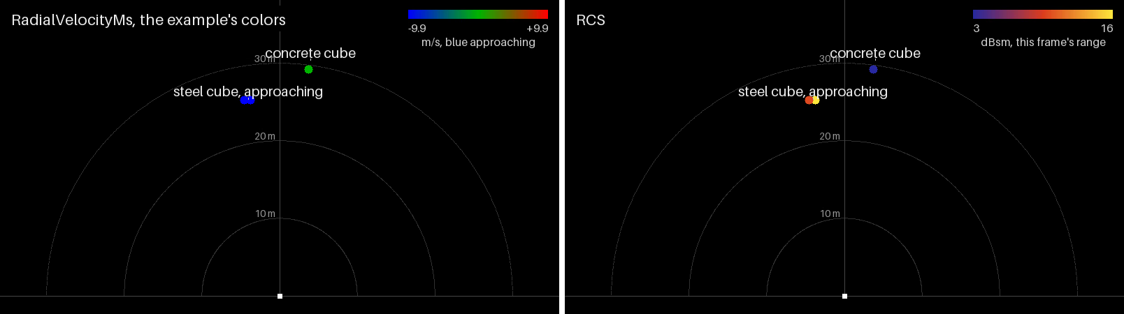
The detections of the radar example scene on step 5 of the example’s run, seen from above, the steel cube approaching at 10 m/s and the concrete cube standing still: left, colored by signed RadialVelocityMs with the example’s mapping, the approaching cube blue and the static one green; right, the same detections colored by RCS from this frame’s minimum to its maximum. The scene is the C example’s copy, which requests RCS.

Related

• USD Attributes — the attributes that shape this output and the scan limits the params report

• Choose Parameter Values — mapping a datasheet to attributes and checking that they reached the model

• Run More Than One Scan Pattern — authoring several scans and verifying the cycle from scanIdx and cycleCnt

• Validate a Parameterization — the checks that read these params and detections

• Simulate Moving Targets — the motion BVH and radial velocity from a moving scene