
Validate a Parameterization#
Validate a Radar generic wpmDmat profile in controlled scenes before using it in a full scenario. Start with a configuration that produces detections.
Before you start, you should have chosen the values on the prim
(Choose Parameter Values), given the radar one scan configuration per operating
mode (Run More Than One Scan Pattern) and created the renderer so that moving
targets produce radial velocity (Simulate Moving Targets). You should know how a
radar frame is read back, bounding by Counts and testing the VALID bit
(Outputs, and Sensor Outputs
for the rule every point cloud follows), and where each attribute is explained
(USD Attributes).
Validation workflow#
One controlled scene, one thing changed at a time, many frames per measurement:
Build a small scene with one reference target at a known range and angle.
Record the detections across many frames, not one.
Change exactly one parameter group.
Record again with the same scene, motion and material assignments, from the same starting point and with the same steps.
Compare the distributions.
Apply this procedure to the seven validation scenarios below, in order.
Method#
Validate each scan configuration in a small scene with known geometry and motion before evaluating a full traffic scenario. This makes discrepancies easier to isolate.
Compare distributions over multiple frames. Sampling, measurement noise and CFAR filtering can change the detection count, so a single-frame comparison cannot reliably identify the effect of a parameter edit. See output variation.
Change one parameter group at a time, and hold everything else fixed.
Retain the scene, motion and material assignments so results remain
comparable. The model takes no seed. Its noise starts from a fixed, built-in
point when the RenderProduct is first stepped and again after
reset() (ovrtx_reset() in C). It advances
with every frame the model traces. Keep the step sequence the same between
recordings. If two things change between runs, or the scene is re-authored
between them, you cannot tell which change caused a difference.
Check coordinates and coverage, resolution and accuracy, Doppler and ambiguity, materials and antenna response, and multipath before tuning CFAR and noise. Errors in these inputs can otherwise be mistaken for filtering errors. Check timing and scan cycling after validating the measurements.
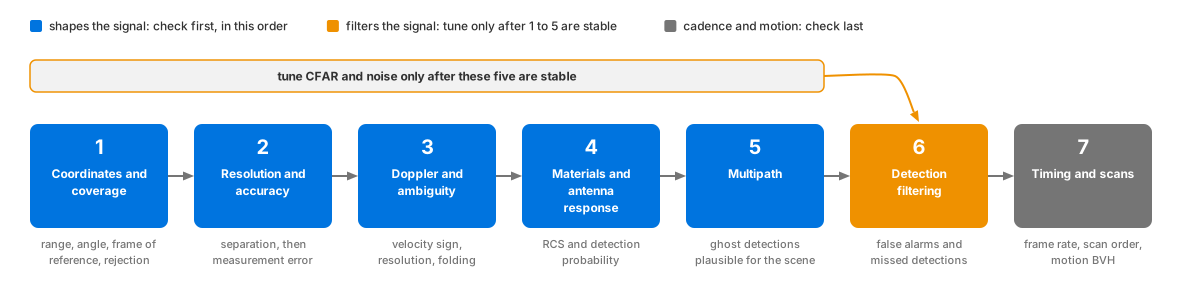
The seven checks in dependency order. Each check assumes the ones to its left hold: detection filtering comes after everything that shapes the signal it filters, and timing comes last, because a scan has to measure correctly before its cadence matters.#
Read scanIdx and the scan-limit parameters alongside the detections.
They report the scan configuration, maximum range, velocity interval and
angular limits. Request Coordinates, RCS and RadialVelocityMs on
the PointCloud RenderVar. Counts and Flags are always included;
see channels.
Note
None of the checks rests on per-detection timing: a radar frame carries none, as Timestamps explains.
Validation scenarios#
Run each scenario in order and compare observations with the stated criteria.
Checks that expect a target require valid detections; a published scan with
Counts[0] == 0 contains no detections to measure.
1. Coordinates and coverage#
Place one strong reference target at known ranges and at boresight, at the field-of-view edges and just outside the field of view. Verify range, angle, frame of reference and rejection.
With enAngAliasing false, the boresight and edge placements must each
produce detections whose reported range matches the known range. Place the
edge targets just inside the edge: every antenna gain profile is zero outside
the scan’s angular limits, and the default, COSINE_FALLOFF, falls to zero at
the limit itself (antenna).
The placement outside the field of view must produce no detection of the
target. Count detections as Counts, Flags and the detection cap describes, bounding by Counts[0]
and testing the VALID bit; the same section says what a scan that
detects nothing delivers.
Coordinates are reported in the coordinate system and frame the output
attributes select, so confirm those first if the ranges look wrong by a
constant (Output coordinates).
2. Resolution and accuracy#
Place two targets on either side of the published range, velocity or angular separation limit. Test separation independently from measurement error, then enable noise and compare the error distribution.
With measurement noise disabled, vary target separation and placement relative
to bin boundaries. Measure how often the pair resolves across positions and
frames, and compare that result with the device’s acceptance criteria.
Resolution is not a hard separation threshold: binning, return strength and
CFAR filtering all affect the result.
For angular separation in a FAST scan, set cfarMode to 4D first:
under the default 2D two targets in the same range-velocity cell come back
as one whatever the angular resolution
(cfarMode). Then
enable the corresponding noise attribute (noise): the spread of the reported
values must widen, and it must widen where you authored it. For a target at
boresight, expect the spread of the reported angle to match the standard
deviation you authored; towards the edge of the field of view it is wider.
Noise authored on range that widens the azimuth distribution instead means the
attribute is not the one you think it is.
3. Doppler and ambiguity#
Move a target at known radial velocities below and beyond the scan’s unambiguous velocity. Verify velocity sign, resolution and folding. Repeat with transverse motion to distinguish speed from radial velocity.
Below the limit, RadialVelocityMs must match the known radial velocity,
with the sign the geometry implies: an approaching target reads negative
(RadialVelocityMs).
Beyond it, the value must fold back into the scan’s unambiguous interval, a
plausible reading at the wrong velocity rather than a dropped detection. Which
interval that is depends on the scan’s datacubeMode. A FAST scan folds
into the symmetric interval the frame reports as minVelMps to
maxVelMps; read it from each frame rather than predicting it, because the
active entry of maxVelMpsSequence advances only when that scan fires
(velocity cycle).
A WAVEFORM scan reports the bounds derived from its selected
chirpRepetitionTimeSequence entry, the sensor’s waveLengthMm and its
other chirp attributes
(aliasing). Purely
transverse motion at the same speed must not produce the same Doppler; if it
does, the motion is not reaching the trace (Simulate Moving Targets).
4. Materials and antenna response#
Sweep a reference target across range, incidence angle and field of view.
Compare RCS and detection probability for calibrated non-visual materials and
antenna data. This check needs the RCS channel on the RenderVar.
RCS must vary across the sweep. An RCS distribution that is identical
for two non-visual materials the radar distinguishes, or flat across incidence
angle, means the material assignment or the antenna gain data is not being
applied, not that the sensor is insensitive. Pick two different base
materials, such as steel against concrete as the runnable radar
examples do. Non-Visual Sensor Materials covers how the
labels are authored, and antenna the gain data.
5. Multipath#
Add a ground plane, wall or other strong reflector and compare direct-path
detections with traceTreeDepth values appropriate to the intended scenario.
Confirm that any ghost detections are physically plausible for the scene.
Raising traceTreeDepth is what allows detections at ranges longer than the
direct geometric distance to the target, because the reported range is half the
round-trip propagation distance; whether any appear depends on the scene
geometry and the material response (traceTreeDepth). It can also cost a
direct-path detection; the CFAR note explains why. And a scan keeps at
most 2500 detections (the detection cap), so when Counts[0] is
2500 a direct-path detection can be among those dropped. A direct-path
detection that disappears must be explained by indirect energy you can place
in or next to its cell, or by a scan at the cap; one that cannot be is a fault.
Each added detection has to be explainable by a path you can draw in the scene;
one that cannot be is a parameterization to reject, not a result to keep.
6. Detection filtering#
Adjust CFAR and noise only after geometry, materials, antenna response and resolution are stable. Compare false alarms and missed detections against recordings or explicit acceptance criteria.
Count false alarms and missed detections over many frames, in a scene where
every reflector is known, and compare both against a criterion written down
before the run. An empty scene is not a false-alarm test for this model.
Raising cfarOffset should reduce false alarms and increase missed
detections; a change that moves both in the same direction means something
earlier in the list is still unstable. See CFAR for threshold formation, control
definitions and the limits of empty-scene testing.
7. Timing and scans#
Verify the frame rate and the scan order for every configured scan. For moving sensors or targets, confirm that the renderer’s motion BVH is on and that the expected time-dependent geometry and Doppler appear.
Frames must arrive at the authored omni:sensor:frameRate when you step at
the scan period, once omni:sensor:startTime has passed. A step without a
radar firing returns no radar frame; a completed scan with no detections
still returns a frame with Counts[0] == 0 (empty scans). The scan index, read from
each PointCloud’s scanIdx param, must then cycle through the configured
scans in lexicographic instance order, with the scan limits changing in step;
Run More Than One Scan Pattern gives that check in full. For a nonzero
timeOffsetUsec, check that timestampNs includes the delay and that a
moving target’s position matches that time. A step that fires no scan must
leave the pending scan and its ambiguity entry unchanged.
For motion, the Radar generic wpmDmat model needs an active motion BVH, with
AUTO or ENABLE (Motion BVH); create the renderer as
Simulate Moving Targets shows, and confirm it
before evaluating target Doppler.
The question at this step is whether the motion reaching the trace is the motion you intended. Both runnable radar examples animate a steel cube toward the radar and print the radial-velocity interval of each step; Simulate Moving Targets describes the scene and the printed summary. A target you have animated toward the sensor must move the printed interval away from zero, on the negative side; if it stays at zero on steps that carry real detections, check whether scene updates are reaching rendering. Over several steps, check that valid detections are present and the approaching target has negative radial velocity. Distinguish that target from stationary panels; a nonzero velocity somewhere in the frame is not enough to validate its sign or magnitude.
Verification#
Validate every scan configuration against known scene geometry, motion and the device’s published limits. Follow the comparison procedure: change one parameter group at a time and record distributions across repeated frames with a consistent step sequence. Investigate failed checks before using the profile in a larger scenario. Choose Parameter Values identifies the relevant controls.
Potential issues#
Every check produces zero detections: first distinguish steps with no radar frame from published scans with
Counts[0] == 0. The latter are completed acquisitions that detected no targets; see empty scans. For nonempty scans, bound reads byCounts[0]and check theFlagsVALIDbit per Counts, Flags and the detection cap. Confirm that the authored limits reached the model per the reach-the-model check.Results change between two runs you believe are identical: the scene, the motion or the material assignments moved, or the runs did not start from the same point or take the same steps. Refer to holding everything else fixed.
A single frame looks right and the aggregate does not, or the reverse: one frame is not a measurement once noise is enabled. Refer to comparing distributions.
CFAR settings that worked in one scene fail in another: they were tuned before materials and antenna response were stable. Refer to the order of the checks.
Detections appear at plausible but wrong ranges, angles or velocities: range or angular aliasing is enabled, or the target is faster than the scan’s unambiguous velocity, which a
FASTscan folds without a switch. That is folding, not error, and it belongs in the parameterization only when the real operating mode has the same ambiguity (aliasing).Only one scan ever appears to be validated: the scan index, the
scanIdxparam of eachPointCloud, is not advancing. Refer to Run More Than One Scan Pattern.A target you animated shows no motion effects, and no error was logged: the renderer was created without the motion BVH, so the radar ran without it. Refer to Simulate Moving Targets.