USD Attributes

The Camera generic core model is instantiated by applying OmniSensorGenericCameraCoreAPI to a Camera prim. Unlike the non-visual models, it has no sensor prim type of its own: the schema can only be applied to a Camera, so the sensor is the camera you already render through, and the camera’s own intrinsics (focal length, aperture, clipping range) keep governing the rendered view exactly as before. Those intrinsics are the UsdGeomCamera attributes of USD Camera Attributes; what the model does and does not read of the camera is on the Overview.

This page explains what the model’s own attributes mean: their units, the order in which they act within a stage, and how they relate to one another. They are grouped as the model groups them: color correction, color filter array, sensor noise, companding and ISP. Types, defaults and allowed tokens are not repeated here; the generated OmniSensorGenericCameraCoreAPI table in Sensor API Schemas lists every attribute with its type, default and doc string. The Camera single-view stereo depth model publishes its own attribute set under its own namespace; see its USD attributes.

Namespaces

Two namespaces, and one of them is a case trap. The attributes that identify which model to load, and schedule it, sit in plain omni:sensor:, because every sensor model shares them; Sensor Configuration describes that shared set. Everything this model reads is omni:sensor:core:*, with a lower-case core.

One capital-C attribute does belong on a camera, and it is not an attribute of this model: omni:sensor:Core:partialOutputs is the camera’s exposure-portion delivery policy, whether an exposure that spans several steps delivers every portion or only the completed frame, and Rolling Shutter and Sensor Scheduling describe it.

This page writes leaf names under omni:sensor:core:: read colorCorrectionBlack as omni:sensor:core:colorCorrectionBlack.

Identification and scheduling

Applying the schema authors the shared identity attributes: omni:sensor:modelName as "CameraCore", omni:sensor:modelVendor as "NVIDIA" and omni:sensor:marketName as "Generic". Model identity explains what the three decide in general. On a Camera they are read together: the pipeline recognizes this model by exactly the set the schema writes, so keep all three at those values. What runs the pipeline on a product is requesting the model’s output names on a product whose camera carries this schema, as the section on what enables the pipeline in Outputs explains.

Three shared attributes schedule the sensor; Shared attributes on Sensor Configuration defines them. This schema sets omni:sensor:frameRate to (30, 1), so applying it schedules the camera at 30 Hz, however often you step; author (0, 1) to leave the camera unscheduled and render on every step. omni:sensor:startTime and omni:sensor:frameLimit keep the shared defaults. Frame rate, step and delivery on Sensor Scheduling says what the rate does to scheduling and delivery.

omni:sensor:frameRate cannot be changed on a running sensor; the schema’s own declaration says so. It is the only attribute of this schema class that carries such a note; Runtime Parameter Updates covers how to tell for the others.

Authoring example

The fragment below applies the schema to a camera and writes out a few of the schema defaults, from three of the groups, so you can see where they live: the frame rate, the full-well level and the white balance of color correction, the output format of the color filter array, and the two dark-shot noise parameters.

def Camera "camera_core" (
    prepend apiSchemas = ["OmniSensorGenericCameraCoreAPI"]
)
{
    double2 omni:sensor:frameRate = (30, 1)
    float omni:sensor:core:colorCorrectionFullwellBlack = 1.0
    float[] omni:sensor:core:colorCorrectionWhiteBalance = [1.0, 1.0, 1.0]
    token omni:sensor:core:colorFilterArrayOutputDataTypeFormat = "UINT32"
    float omni:sensor:core:noiseDarkShotNoiseGain = 10.0
    float omni:sensor:core:noiseDarkShotNoiseSigma = 0.5
}

Apply the schema: the model runs only on a camera that carries it, and requesting one of the model’s outputs on the RenderProduct is what starts the pipeline, as What enables the pipeline explains. Sensor Configuration shows how to apply a schema in USDA and in Python, and Shape an Image Like a Camera Sensor walks through the whole task from schema to verified output.

The attribute groups

The sequence of operations is fixed; what you author decides how each behaves. You do not wire a graph by hand: the attributes on the camera prim configure a pipeline whose shape is already set, and Outputs gives the order of the stages and what each one publishes. The one exception is the ISP stage, which runs a program you supply rather than one assembled from attributes. The groups, by the operation they configure: color correction (black level and full-well normalization, the response scale, the 3×3 matrix and the white balance), the color filter array (the four weight triples of the 2×2 mosaic, its semantic label, its output format and the maximal value that puts codes in sensor units), sensor noise (the dark-shot parameters and the high-dynamic-range combination table), companding (the curve, its two pedestals and the code’s alignment within the output integer) and the ISP (the program, and the raw format and padding mode that describe the companded codes to it).

Two of the groups reshape the element formats in addition to changing the pixels values: colorFilterArrayOutputDataTypeFormat changes the element type of the color filter array tap, the companding curve decides whether the companded image, OmniCameraSensorPreIsp, is written as 16- or 32-bit integers. Additionally, an empty ispSmodelCameraProgram leaves the two post-ISP outputs without an image. Outputs lists all three beside the per-stage format table.

Color correction

Color correction is where the rendered image is made to look like what this sensor would have measured rather than what a neutral observer would see. Real photosites do not have the spectral response of the render’s primaries, so a 3×3 matrix maps render primaries onto sensor primaries, and per-component gains account for the illuminant and for the sensor’s own digital-number scale. The stage reads the linear high-dynamic-range input (Configure the Input Image) and writes a color image of the same shape; its output format is fixed, four-component 16-bit float, as the format table on Outputs lists.

Within the stage the operations are ordered, and the first is gated:

1. Black level and full-well normalization, only while colorCorrectionApplySaturation is true, which is not the default. colorCorrectionBlack, the black floor in the input’s units, is subtracted from every component and the result is floored at zero; the result is then divided by colorCorrectionFullwellBlack, the input level at which the photosite saturates, and clamped at 1. While colorCorrectionApplySaturation is false, colorCorrectionBlack and colorCorrectionFullwellBlack have no effect, so authoring either one alone changes nothing you can measure.

2. Sensor response scale. colorCorrectionSensorResponseScale multiplies every component, so the stage’s output is linear in the authored value.

3. The 3×3 matrix. It is authored as nine separate scalars, colorCorrectionMatrixRr through colorCorrectionMatrixBb, not as one matrix-valued attribute. The naming is output from input: colorCorrectionMatrixRg is the green input’s contribution to the output red, and Rr, Rg and Rb together form output red. The identity, ones on the diagonal and zeros elsewhere, is the default and leaves color untouched.

4. White balance. colorCorrectionWhiteBalance is three gains in R, G, B order, applied after the matrix. It compensates for the color temperature of the illuminant and can also scale values into the sensor’s digital-number range.

The matrix coefficients and the gains are dimensionless; the black level and the full-well level are in the units of the input image.

Three more attributes of this group, colorCorrectionRedBlueSwap, colorCorrectionOutputFloat16 and colorCorrectionOutputFloat32, have no effect in ovrtx: the stage writes four-component 16-bit float regardless, and authoring them is not an error. Limitations lists them.

Attribute	What it does
colorCorrectionApplySaturation	Switches on the black level and full-well normalization step; false by default. While false, the next two attributes have no effect.
colorCorrectionBlack	Black floor subtracted from every component, in the units of the input image; the result is floored at zero. Read only while colorCorrectionApplySaturation is true.
colorCorrectionFullwellBlack	Input level at which the photosite saturates, in the units of the input image; the black-subtracted value is divided by it and clamped at 1. Read only while colorCorrectionApplySaturation is true.
colorCorrectionSensorResponseScale	Dimensionless multiplier applied to every component; the stage’s output is linear in it.
colorCorrectionMatrixRr to colorCorrectionMatrixBb	The nine dimensionless coefficients of the 3×3 matrix from render primaries to sensor primaries, named output from input; the identity by default.
colorCorrectionWhiteBalance	Three dimensionless gains in R, G, B order, applied after the matrix.
colorCorrectionRedBlueSwap, colorCorrectionOutputFloat16, colorCorrectionOutputFloat32	No effect in ovrtx; the stage writes four-component 16-bit float regardless.

Color filter array

This is the first of the two groups that reshape the element formats.

This stage is the mosaic filtering that Why the color filter array matters on Author a Color Filter Array explains: it takes the color-corrected RGBA image and produces one sensor code per pixel, exactly as the physical mosaic over the photosites would.

The stage encodes the RGBA input into a single-component color filter array image.

The pattern is four RGB weight triples, one per position in the 2×2 block. colorFilterArrayCfaCf00 is the top-left position, colorFilterArrayCfaCf01 the top-right, colorFilterArrayCfaCf10 the bottom-left and colorFilterArrayCfaCf11 the bottom-right. Each is three floats, the weights of red, green and blue, and the code written for a pixel is the weighted sum of the pixel’s red, green and blue, scaled by colorFilterArrayMaximalValue. A triple of [0, 1, 0] is a green filter, [1, 0, 0] a red one, and [1, 1, 1] is a clear pixel, no filter at all.

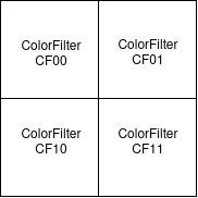
The four positions of the 2×2 block and the attribute that carries each one’s weight triple.

Because the weights are independent, any 2×2 mosaic can be expressed. The shipped defaults are green, red, blue, green reading across and down, a GRBG Bayer pattern, one of the four orderings of the classic arrangement below, and the default of the semantic token, GRBG, agrees with them.

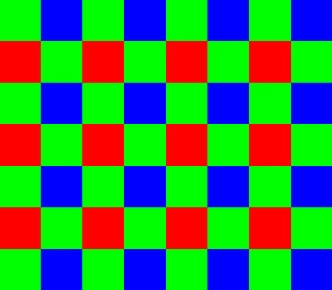
A Bayer mosaic; the shipped default GRBG is one of its four orderings.

The semantic token names the pattern; it does not create it. colorFilterArrayCfaSemantic records which pattern you intended, and takes one of nine values: RGGB, GRBG, BGGR, RCCB, CRBC, BCCR, RCCC, CCCR or CRCC. The image is produced from the four weight triples alone, so the token is a label for whoever reads the scene, not an input to the stage: setting it to RCCB while leaving Bayer weights in place gives a Bayer image labeled RCCB, and the values must agree. Change the weights and the token together, always; Author a Color Filter Array gives the triples for each pattern. An all-clear arrangement, CCCC, all four positions clear and effectively monochrome, has no token of its own; express it with four [1, 1, 1] triples. Why the color filter array matters on Author a Color Filter Array explains what the choice of mosaic trades off, low-light sensitivity against color separation.

The output format changes this stage’s element type only. colorFilterArrayOutputDataTypeFormat is UINT32 by default or FLOAT32. With UINT32 each code is written as an unsigned integer, rounded down; with FLOAT32 the fractional code is kept. The noise stage converts FLOAT32 codes back to unsigned integers before it adds noise, so every later stage works on integer codes either way and the float representation ends at OmniCameraSensorPostCfa; the format table on Outputs shows the consequence for each tap.

The maximal value puts the result in sensor-code units. colorFilterArrayMaximalValue multiplies the weighted sum. If the incoming image is normalized to 1, it is the maximal code the sensor can produce: 16777215 for a 24-bit internal range, 1048575 for 20 bits, 1 for pass-through. If the incoming image is not normalized, it is simply a linear multiplier; either way it is a multiplier, not a clamp. The attribute is declared float so that a non-integer radiometric scale can be authored as readily as a bit-depth maximum. A 32-bit float represents integers exactly only up to 2²⁴, so the 24-bit default is held exactly and a larger integer maximum may be rounded.

Attribute	What it does
colorFilterArrayCfaCf00, colorFilterArrayCfaCf01, colorFilterArrayCfaCf10, colorFilterArrayCfaCf11	The RGB weight triple of the top-left, top-right, bottom-left and bottom-right position of the 2×2 block; a pixel’s code is its red, green and blue weighted by the triple of its position, scaled by the maximal value. The defaults form a GRBG Bayer pattern.
colorFilterArrayCfaSemantic	Token naming the pattern you intended, one of nine; a label for whoever reads the scene, not an input to the stage.
colorFilterArrayOutputDataTypeFormat	UINT32 writes each code as an unsigned integer, rounded down; FLOAT32 keeps the fractional code. Changes this stage’s element type only.
colorFilterArrayMaximalValue	Multiplier on the weighted sum, not a clamp; with an input normalized to 1 it is the sensor’s maximal code (16777215 for 24 bits).

Sensor noise

Two noise sources are modeled, and they have different physical causes. Photon shot noise is the randomness of photon arrival itself: it grows with the signal, so a bright pixel is noisier in absolute terms and cleaner in relative terms. Dark shot noise comes from thermally generated carriers and is present whether or not light is: it does not scale with the signal, which is why it dominates in shadows and in short exposures. Both are random from frame to frame.

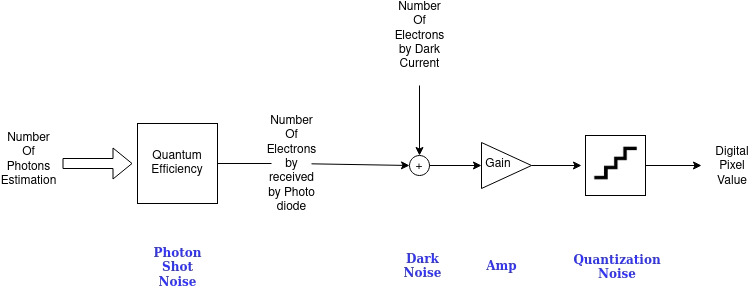
The sensor noise chain; the model implements its photon-shot and dark-shot terms.

Only these two are modeled; spatial noise is not. Fixed-pattern noise, photo-response non-uniformity (PRNU) and dark-signal non-uniformity (DSNU) are per-photosite offsets and gains that do not change from frame to frame, the texture a real sensor imprints on every image. None of them is simulated, so fixed-pattern artifacts do not appear in this output. Limitations lists this as a limit of the model.

Two attributes control dark shot noise, and neither controls photon shot noise. noiseDarkShotNoiseSigma is the standard deviation of the dark-shot distribution, in sensor codes, and noiseDarkShotNoiseGain scales it; the two multiply, so the defaults of 0.5 and 10.0 give a dark-shot term with a standard deviation of five codes. Photon shot noise has no attribute at all, because its magnitude follows from the signal: its standard deviation is the square root of the pixel’s code, which is what makes it shot noise rather than a tunable. Both terms are added to the code and the sum is floored at zero. Because the photon term is the square root of the code, the scale you choose with colorFilterArrayMaximalValue sets its absolute size: about 4096 codes at the 24-bit maximum of 16777215, one code at a code of 1, and none at a code of 0.

High-dynamic-range sensors capture in zones, and the noise model follows them. An HDR sensor covers a wider range than one exposure can by combining several captures taken at different gains and stitching them into one code space. Noise is not uniform across that stitched range: a code that came from the high-gain capture carries less real signal, and therefore more relative noise, than the same code from the low-gain capture. noiseHdrCombinationData describes that structure as a list of pairs, one per zone in order of increasing code: the zone’s gain, then its upper bound in code space. For each pixel the model takes the first zone whose bound exceeds the pixel’s code, or the last zone when none does, divides the code by that zone’s gain to recover the underlying signal, computes both noise terms against that, and scales the result back by the gain. A table with one pair or none means the plain single-exposure path. The shipped default has three zones; the generated table in Sensor API Schemas lists it.

Attribute	What it does
noiseDarkShotNoiseSigma	Standard deviation of the dark-shot distribution, in sensor codes, before the gain.
noiseDarkShotNoiseGain	Dimensionless scale on that standard deviation; the product of the two is the dark-shot term’s standard deviation in codes, five with the defaults. Photon shot noise has no attribute; it follows from the code.
noiseHdrCombinationData	The HDR zones as pairs of gain and upper bound in code space, in increasing code order; one pair or none means the single-exposure path.

Companding

This is the second of the two groups that reshape the element formats.

Companding compresses the sensor’s wide internal range onto the narrower RAW width it transmits, with a piecewise-linear curve that the ISP later reverses (compress and expand); the Overview explains why a sensor does this rather than truncate.

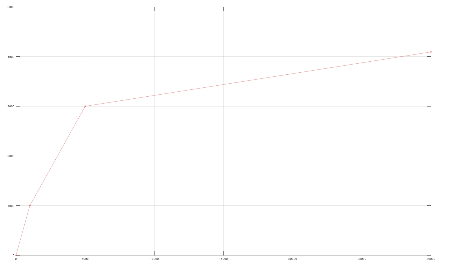
A piecewise-linear companding curve mapping a wide internal range onto RAW12.

The curve is authored as its knee points. compandingLinearCompandCoeff is a list of (x, y) pairs, where x is the uncompressed internal value and y the compressed output code. Between two knees the mapping is linear; from the last knee on, the output clamps to that knee’s y; the result is rounded to an integer code. Author at least two pairs, in increasing x. The schema ships a 17-point curve that maps 0 to 16777215 onto 0 to 4095, which is 24-bit internal onto RAW12; Sensor API Schemas has it written out, and Compand to a RAW Format and Run the ISP shows how to build a curve for another width.

A pedestal is a constant offset, and there are two of them. compandingPrePedestal is added to the value before the curve is applied, in internal units; compandingPostPedestal is added to the code after the curve, in output codes, before the alignment shift. Negative values count as zero. Real sensors carry a pedestal so that noise around black does not clip at zero and become one-sided.

Alignment determines the code’s bit positions in the output integer. A 12-bit code can occupy the least or most significant 12 bits of a 16-bit unsigned integer, depending on the receiver’s requirements. compandingAlignment specifies the position of the code’s most significant bit in the output integer, counting from 0 at the least significant bit. Bit positions range from 0 to 15 for a 16-bit integer and 0 to 31 for a 32-bit integer. The stage derives the shift from that position and the number of bits needed for the curve’s largest output. For a RAW12 curve with a maximum output of 4095, compandingAlignment = 15 shifts the 12-bit code left by 4 into bits 15 to 4; compandingAlignment = 11 leaves it unshifted in bits 11 to 0. An alignment below the code width minus one shifts the code right and discards its least significant bits. The post-pedestal is excluded from the shift calculation, so ensure the shifted value, including the post-pedestal, fits in the output integer. The diagram beside Choose the alignment draws both layouts.

The curve’s largest output determines the companding output type. The ISP requires 16-bit unsigned integer input. Stay within 16 bits states the rule and what happens to a product that requests both; Limitations records the requirement.

Attribute	What it does
compandingLinearCompandCoeff	The knee points of the curve as (x, y) pairs of internal value and output code, at least two in increasing x; linear between knees, clamped past the last. Its largest y determines the output integer type.
compandingPrePedestal	Constant offset added before the curve, in internal units; a negative value counts as zero.
compandingPostPedestal	Constant offset added after the curve, in output codes, before the alignment shift; a negative value counts as zero.
compandingAlignment	Bit position of the code’s most significant bit in the output integer, counting from 0 at the least significant bit: 0 to 15 for a 16-bit type, 0 to 31 for a 32-bit type.

ISP

The image signal processor undoes what the sensor did, and then some. It expands the companded codes back to a linear range (decompanding), reconstructs three color components per pixel from the mosaic (demosaicing), denoises, and converts to a working color space. The stage produces a YUV image; the final stage of the pipeline decodes it to RGBA, as Outputs describes.

The ISP is not configured by attributes; it runs a program you supply. ispSmodelCameraProgram holds a base64-encoded ISP program, and its schema default is the empty string, so until you author one the stage has nothing to apply and the post-ISP outputs carry no processed image. Outputs describes the consequence for each output, and Compand to a RAW Format and Run the ISP covers obtaining and authoring a program.

Two attributes describe the data the stage is handed rather than what to do with it. ispSmodelSensorRawFormat, one of RAW8, RAW10, RAW12, RAW14, RAW20 or RAW24, says which RAW width the companded codes represent; with the ISP in the pipeline that is one of RAW8 to RAW14, because the full pipeline carries 16-bit codes and a RAW20 or RAW24 code needs more. ispSmodelRawDataPaddingMode, one of NONE, RIGHT or LEFT, specifies the code’s alignment within the input integer. For RAW12 in a 16-bit unsigned integer, LEFT describes a code in bits 15 to 4 with zero padding in bits 3 to 0, matching compandingAlignment = 15. RIGHT describes a code in bits 11 to 0 with zero padding in bits 15 to 12, matching compandingAlignment = 11. NONE specifies no padding. Author both attributes explicitly to match what the companding curve and alignment produce.

Attribute	What it does
ispSmodelCameraProgram	The base64-encoded ISP program; empty by default, so the post-ISP outputs carry no processed image until you author one.
ispSmodelSensorRawFormat	The RAW width the companded codes represent: RAW8, RAW10, RAW12, RAW14, RAW20 or RAW24; one of RAW8 to RAW14 with the ISP in the pipeline.
ispSmodelRawDataPaddingMode	Alignment within the input integer: LEFT indicates a code in the most significant bits, RIGHT in the least significant bits. In both cases, the remaining bits are zero padding. NONE specifies no padding.

Related

• Outputs — the reserved output names, primary outputs and taps, and the per-stage formats these attributes shape.

• How-To — the task pages on the image pipeline, the input image, the color filter array, companding and the ISP.

• Sensor API Schemas — the generated OmniSensorGenericCameraCoreAPI table listing every attribute with its type, default and doc string.