Overview

ovrtx brings Omniverse RTX sensor simulation into C and Python applications. One renderer produces camera images and simulates lidar, radar and acoustic returns from the same OpenUSD scene and materials. Camera images are path-traced in the default mode.

A sensor consists of a USD prim and a request for its outputs. Start with Your First Lidar Sensor to configure a lidar and read its point cloud, or choose a sensor type below.

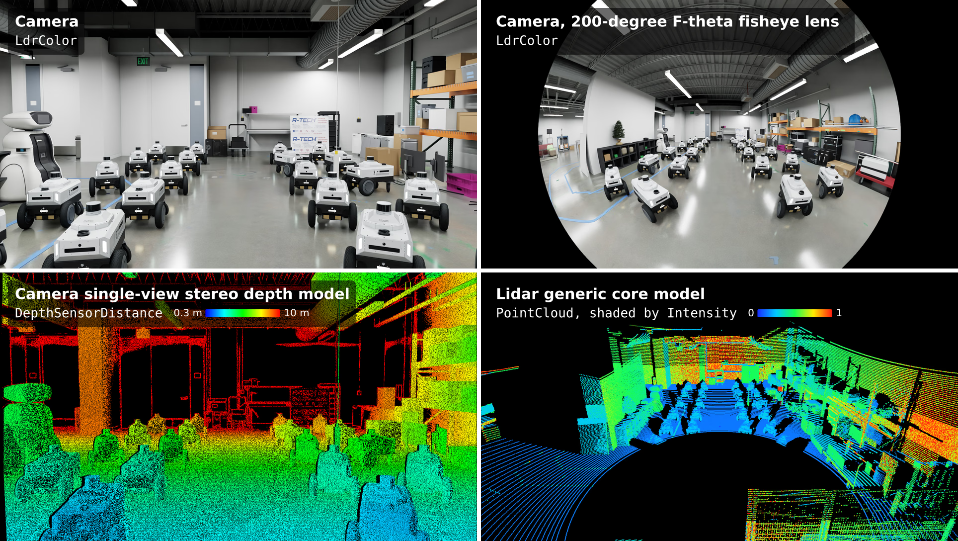
One scene, four sensors on one robot: the camera’s rendered LdrColor image (top left); the LdrColor image of a camera with a 200-degree F-theta fisheye lens (top right); the DepthSensorDistance image of the Camera single-view stereo depth model, 0.3 m blue to 10 m red (bottom left); and the PointCloud of a 128-channel rotary Lidar generic core model, shaded by Intensity and seen from behind and above the sensor (bottom right). The robotics lab is a demonstration scene, not one of the shipped examples.

Sensor types and modalities

Each sensor type produces different data:

• Cameras: images of color, geometry, segmentation and object IDs. These outputs are called arbitrary output variables (AOVs). See Camera Outputs.

• Lidar: point clouds with coordinates, counts, intensity and per-point timing. See the outputs for Lidar generic core or Lidar generic wpm.

• Radar: detections with coordinates, counts, radar cross-section and radial velocity. See Radar Outputs.

• Acoustic: echo amplitude over time. Each waveform records one receiving mount on one channel id. See Acoustic Outputs.

• Raw propagation: electromagnetic or mechanical path contributions, before detector processing. See Generic wpm and its Contributions output.

A RenderProduct requests the outputs you want. Lidar and radar use a composite PointCloud output; acoustic sensors use SignalWays and the Generic wpm model uses Contributions. Their channels are named tensors. Your First Lidar Sensor introduces the shared workflow for configuring sensors and reading outputs.

Non-visual sensors use material labels to calculate surface responses, independently of camera shading. See Non-Visual Sensor Materials.

Cameras

A USD Camera prim defines the view. Its RenderProduct requests color, geometry, segmentation or other camera outputs. See Cameras for camera attributes and outputs, and Render Modes for the three render modes. Real-Time Path Tracing is the default.

Camera sensor APIs add optional processing to these rendered outputs:

• The Camera generic core model applies sensor response, a color filter array, noise, bit-depth compression and image signal processing to a rendered HDR image.

• The Camera single-view stereo depth model simulates stereo depth measurements from one rendered view, without a second camera render.

Apply the corresponding API schema to the same Camera prim and request its outputs on the RenderProduct. A camera can use one of these two sensor schemas, not both. See Visual Sensors for configuration.

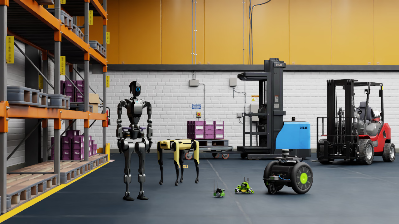
The LdrColor output of a camera product rendered in Real-Time Path Tracing: the robot lineup of the semantic-segmentation example in a warehouse, with path-traced lighting, reflections and shadows.

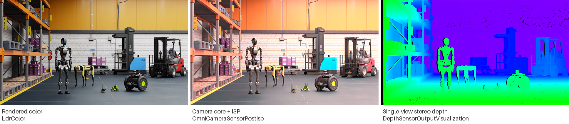
The robot lineup from three cameras at the same pose. Left: rendered LdrColor. Center: OmniCameraSensorPostIsp with a sample camera profile. Right: DepthSensorOutputVisualization, black where no measurement is reported.

Non-visual sensors

Lidar, radar and acoustic sensors trace rays to simulate signals reflected by scene surfaces. See Non-Visual Sensors for the available models and the differences between the Lidar generic core and Lidar generic wpm models.

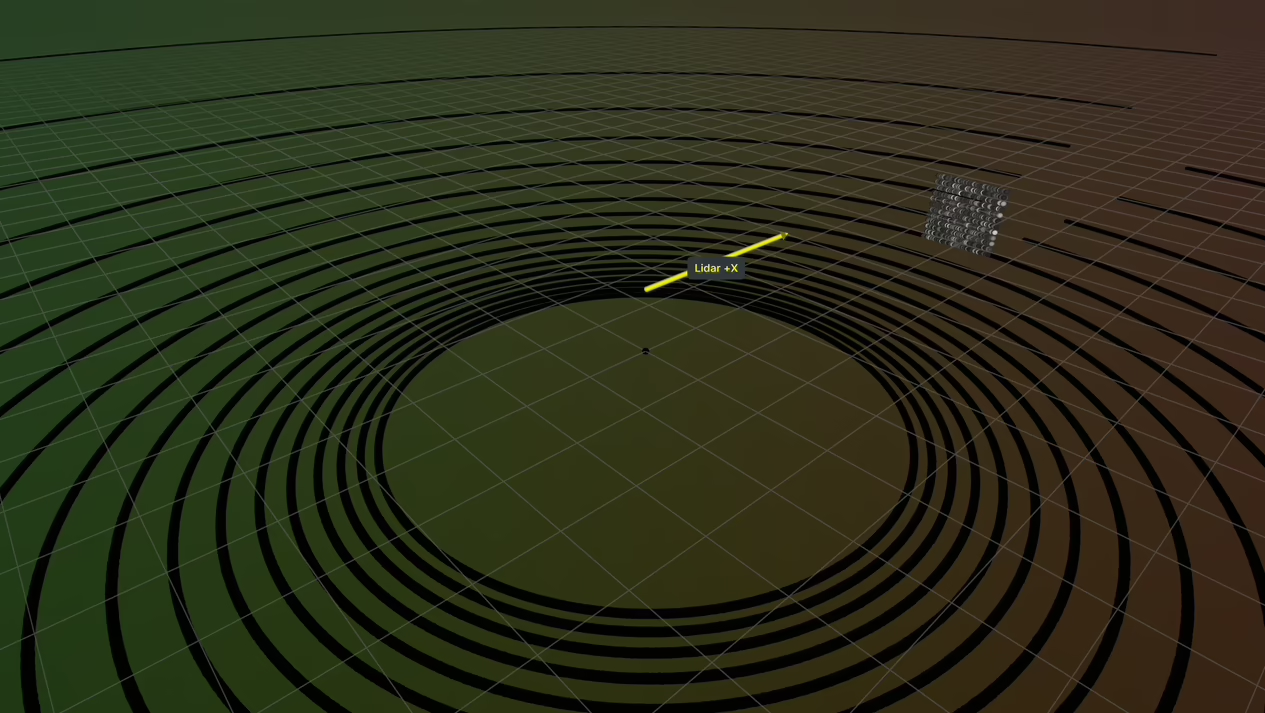
The point cloud of the lidar example, a Lidar generic core model rotated to look along world +X, the arrow in the picture, at an asphalt ground plane and a concrete cube; the scan rings are shaded by Intensity and the cube appears as the dense cluster of points.

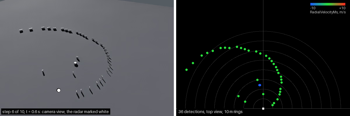
The radar example’s field scene: a Radar generic wpmDmat model watches a steel cube cross a field of steel panels over asphalt. Left, the scene from its preview camera at one step; right, a top view of that step’s detections, colored by signed radial velocity: blue approaches the sensor, green is near zero, red recedes.

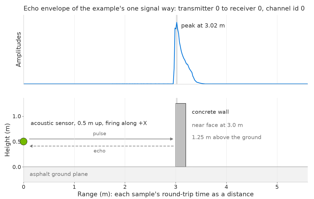
The acoustic example’s echo amplitude plotted against range, calculated from round-trip travel time. Below, the scene uses the same distance axis: the sensor sits 0.5 m above asphalt and fires along +X toward a concrete wall 3 m ahead. The peak marks the wall’s echo.

Documentation guide

Section	Covers
Your First Lidar Sensor	Learn how to configure a lidar, render a scan and read its point cloud in Python or C.
Common Concepts	Sensor configuration, RenderProducts, outputs, runtime changes, capture rates.
Cameras	Camera settings, lens calibration, rolling shutter, render modes, outputs and scene partitions.
Visual Sensors	Camera sensor response, noise, image signal processing and stereo depth.
Non-Visual Sensors	Lidar, radar and acoustic models, their settings and outputs.
Reference	Sensor schemas, lens distortion schemas, and the glossary.
Troubleshooting	Symptoms, causes and fixes and model limitations.

Each model section has an overview, settings, how-tos and output reference. How-tos cover specific tasks. For step-by-step guides to configuring sensors from real-world data, use these tutorials:

• Camera calibration: calibrate a USD camera from checkerboard photographs taken with a physical camera.

• Lidar generic core profiles: build lidar profiles from manufacturer specifications and manuals.

For runnable Python and C code, see the example gallery.

Related

The sections of the Sensors part, in reading order, are in the table above. The pages it does not list:

• Glossary — the shared vocabulary, from AOV and channel to signal way.

• Examples — the runnable Python and C examples, including sensor simulation examples.

• Getting Started in Python and Getting Started in C — installing ovrtx and running the minimal example before you add a sensor.

• Hardware & Driver Requirements — the hardware and the NVIDIA drivers ovrtx runs on.