
Lidar generic wpm model#
The Lidar generic wpm model simulates pulsed time-of-flight lidar. It models pulse propagation, surface interactions and detector response to predict return strength and timing. Paths can cross multiple surfaces, including transmissive ones.
The Lidar generic core model uses geometric ray intersections instead. Choose the wpm model when wave propagation and detector behavior matter. WPM stands for wave propagation model; see the glossary.
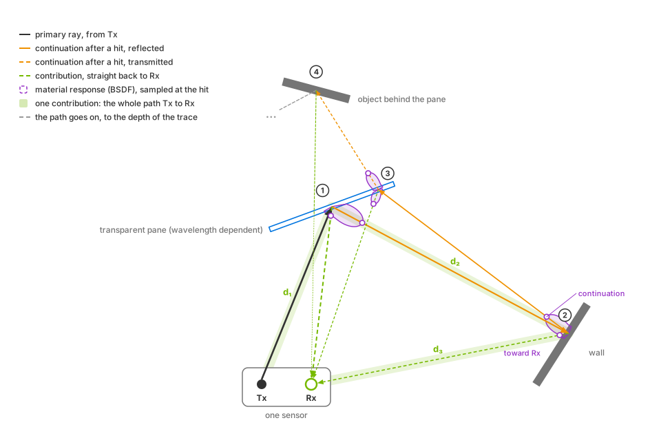
A propagation path from transmitter Tx through a pane, wall and pane to an object behind the glass. Each hit generates one reflected or transmitted continuation and a contribution toward receiver Rx. The highlighted Tx → pane → wall → Rx path has length d₁ + d₂ + d₃, which determines its arrival time. The contribution from behind the pane crosses it again on the return path.#
At each hit, the bidirectional scattering distribution function (BSDF) is evaluated for the continuation and receiver directions. Surface interactions reduce the remaining energy; transmission also depends on wavelength. The diagram shows refraction toward the pane’s normal and traces the path to the configured depth.
Simulation#
A rotary or solid-state scan schedule defines each emitter’s firing time and direction. Each pulse is traced as an idealized ray or a finite-width beam, using the configured power, wavelength, duration, angular jitter and offsets. See Configure a Firing Pattern and USD Attributes.
Surface scattering and transmission use non-visual materials. The model can also use the visual material’s diffuse reflectance, roughness and shading normal. Transmitted paths can produce returns from behind glass; indirect paths can produce ghost returns.
The detector processes arrivals in waveform (default), directDetector
or directMaterial mode. The mode determines how arrivals become returns
and how transmissive surfaces are handled. Each receiver can report up to
omni:sensor:LidarWpm:maxReturns returns per tick; a receiver corresponds
to an emitter row in the firing pattern.
See Choose a Return-Processing Mode for the modes and USD Attributes for
detector controls.
Intensity can report raw detector response or range-normalized apparent reflectivity. This choice changes the reported strength without changing which returns are detected; see Tune Intensity.
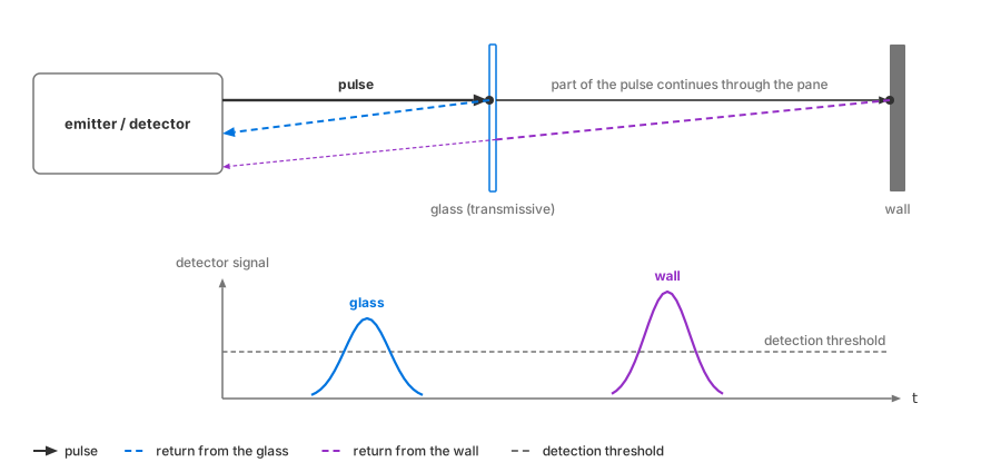
In waveform mode, one pulse can produce returns from a glass pane and the wall behind it, with separate EchoIds. Return strength depends on material, incidence angle and distance; the diagram shows one example.#
Outputs#
The model produces PointCloud outputs with one entry per
return. Eight channels are selectable: Coordinates, Intensity,
TimeOffsetNs, Flags, ChannelId, MaterialId, EchoId and
FiringPatternIndex. See the
channel reference.
Both compact and
dense layouts include
Counts. Compact output also includes two tile tensors. Multiple sensors
on one RenderProduct produce a single
aggregate point cloud.
Capabilities#
Output coordinates can be Cartesian or spherical, in the sensor, world or a custom reference frame. Motion compensation can correct sensor movement during a scan; motion effects require the renderer’s motion BVH. See USD Attributes, Outputs and Output Configuration.
All model attributes support runtime edits. Rejected updates retain the last valid profile; see Retune the Sensor While It Runs. For multiple sensors on one RenderProduct, see Tile Lidars.
Applications#
Use this model to study how materials, beam geometry, detector parameters and multipath propagation affect lidar returns. Examples include returns through glass, strong returns from retroreflective signs, and loss of dark surfaces at long range. Aperture, efficiency, noise, pulse and threshold settings can be varied to evaluate detector response.
For lower-cost geometric point clouds, use the Lidar generic core model. See Performance for controls that affect the wpm model’s cost.
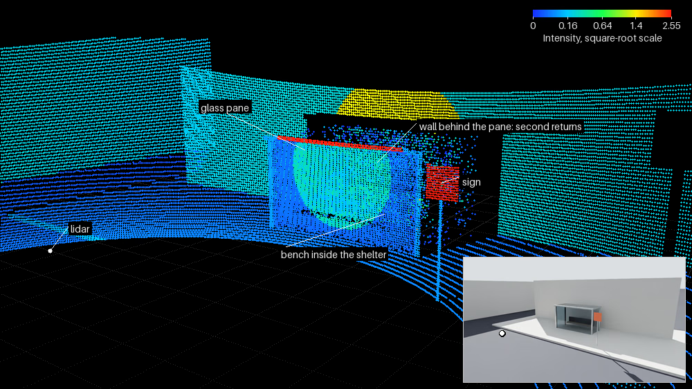
A waveform-mode scan with maxReturns = 2. Points use rangeNormalized intensity, linear mapping and full scale 2.55, displayed on a square-root color scale. The glass pane produces returns, as do the bench and wall behind it. Returns through glass are weaker than direct returns from the exposed wall. The sign and metal frame saturate the scale. The inset shows the same camera view.#
Sensor definition#
Apply OmniSensorGenericLidarWpmAPI to an OmniLidar prim.
The schema sets omni:sensor:modelName = "LidarWpm" to select this model
and supplies the first firing pattern, p001.
To alternate patterns, apply additional instances of
OmniSensorGenericLidarWpmFiringPatternAPI. Name them in firing order:
p002, p003, and so on. Model controls use omni:sensor:LidarWpm:*;
identity and scheduling use the shared sensor attributes.
See USD Attributes and model identity.
Create a RenderProduct with a PointCloud RenderVar, then load, step and read
it as in Your First Lidar Sensor. This model has no runnable project in the
example gallery. Instead, start from the complete
rotary scene in Configure a Firing Pattern; the other how-tos build on it.
The following scene defines a sensor, its p001 firing pattern and a
RenderProduct requesting PointCloud:
#usda 1.0
(
    metersPerUnit = 1
    timeCodesPerSecond = 10
    upAxis = "Z"
)

def Xform "Sensor"
{
    def OmniLidar "Lidar" (
        prepend apiSchemas = ["OmniSensorGenericLidarWpmAPI"]
    )
    {
        token visibility = "invisible"
        double2 omni:sensor:frameRate = (10, 1)
        token omni:sensor:LidarWpm:scanType = "rotary"
        float omni:sensor:LidarWpm:rotPatternFiringResDeg = 1
        uint omni:sensor:LidarWpm:maxReturns = 2

        float[] omni:sensor:LidarWpm:firingPattern:p001:azimuthDeg = [0, 0]
        float[] omni:sensor:LidarWpm:firingPattern:p001:elevationDeg = [-1, 1]
        uint[] omni:sensor:LidarWpm:firingPattern:p001:fireTimeNs = [0, 1000]
        uint[] omni:sensor:LidarWpm:firingPattern:p001:channelId = [1, 2]
        uint[] omni:sensor:LidarWpm:firingPattern:p001:rangeId = []
    }

    def Scope "Outputs"
    {
        def RenderProduct "Product"
        {
            rel camera = </Sensor/Lidar>
            rel orderedVars = [</Sensor/Outputs/PointCloud>]
        }

        def RenderVar "PointCloud"
        {
            uniform string sourceName = "PointCloud"
            token[] channels = []
        }
    }
}
from pxr import Gf, Sdf, UsdGeom, UsdRender

UsdGeom.SetStageMetersPerUnit(stage, 1.0)
UsdGeom.SetStageUpAxis(stage, UsdGeom.Tokens.z)
stage.SetTimeCodesPerSecond(10)
UsdGeom.Xform.Define(stage, "/Sensor")
lidar = stage.DefinePrim("/Sensor/Lidar", "OmniLidar")
lidar.AddAppliedSchema("OmniSensorGenericLidarWpmAPI")
UsdGeom.Imageable(lidar).CreateVisibilityAttr(UsdGeom.Tokens.invisible)
lidar.CreateAttribute("omni:sensor:frameRate", Sdf.ValueTypeNames.Double2, custom=False).Set(Gf.Vec2d(10, 1))
lidar.CreateAttribute("omni:sensor:LidarWpm:scanType", Sdf.ValueTypeNames.Token, custom=False).Set("rotary")
lidar.CreateAttribute("omni:sensor:LidarWpm:rotPatternFiringResDeg", Sdf.ValueTypeNames.Float, custom=False).Set(1)
lidar.CreateAttribute("omni:sensor:LidarWpm:maxReturns", Sdf.ValueTypeNames.UInt, custom=False).Set(2)

# The main schema brings the first pattern instance, p001: author only its arrays.
pattern = "omni:sensor:LidarWpm:firingPattern:p001"
lidar.CreateAttribute(f"{pattern}:azimuthDeg", Sdf.ValueTypeNames.FloatArray, custom=False).Set([0, 0])
lidar.CreateAttribute(f"{pattern}:elevationDeg", Sdf.ValueTypeNames.FloatArray, custom=False).Set([-1, 1])
lidar.CreateAttribute(f"{pattern}:fireTimeNs", Sdf.ValueTypeNames.UIntArray, custom=False).Set([0, 1000])
lidar.CreateAttribute(f"{pattern}:channelId", Sdf.ValueTypeNames.UIntArray, custom=False).Set([1, 2])
lidar.CreateAttribute(f"{pattern}:rangeId", Sdf.ValueTypeNames.UIntArray, custom=False).Set([])

stage.DefinePrim("/Sensor/Outputs", "Scope")
product = UsdRender.Product.Define(stage, "/Sensor/Outputs/Product")
product.GetCameraRel().SetTargets(["/Sensor/Lidar"])
product.GetOrderedVarsRel().SetTargets(["/Sensor/Outputs/PointCloud"])
point_cloud = UsdRender.Var.Define(stage, "/Sensor/Outputs/PointCloud")
point_cloud.GetSourceNameAttr().Set("PointCloud")
# An empty channel list requests every channel the model produces.
point_cloud.GetPrim().CreateAttribute("channels", Sdf.ValueTypeNames.TokenArray, custom=False).Set([])
Comparison with the core model#
Both lidar models use OmniLidar prims. The applied API schema selects the
model through omni:sensor:modelName; see
model identity.
The wpm model uses omni:sensor:LidarWpm:* controls and ignores
omni:sensor:Core:* controls. See USD Attributes.
Configuration and outputs#
Use USD Attributes for controls, bounds and costs, and How-To to configure a working sensor. Read Outputs before consuming point clouds: it defines compact and dense layouts, tiled aggregates, coordinate frames and empty startup output.