Radar generic wpmDmat model#

The Radar generic wpmDmat model simulates radar detections with position, radial velocity and radar cross section (RCS). Positions are spherical by default, with Cartesian output also available (Outputs).

wpmDmat means Wave Propagation Model Detection Matrix. The model traces propagation paths into a range–velocity–azimuth–elevation detection matrix, then extracts detections using a constant false alarm rate (CFAR) threshold. See the glossary for these terms.

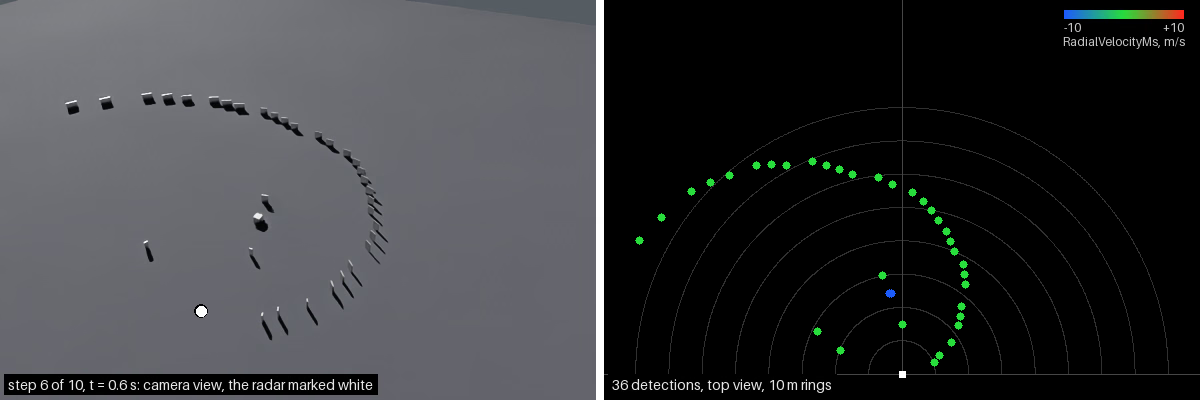
Two panels side by side. Left, the radar example's field scene from its preview camera: steel panels on an arc, a steel cube crossing the field, the radar marked with a white dot. Right, a top view of the same step's detections over 10 m range rings, colored by signed radial velocity: the cube's blue, the panels' green. — Radar 1 m above asphalt, observing a steel cube moving among 33 steel panels. Left: camera view. Right: detections on 10 m range rings, colored by signed radial velocity. Blue approaches, green is near zero and red recedes.#

Simulation#

The model traces paths with multiple surface interactions. Each interaction can contribute energy to the receiver, producing arrivals with different strengths and delays.

Detection processing#

FAST mode maps traced arrivals directly into detection-matrix bins. WAVEFORM mode computes the matrix from sampled waveforms. CFAR processing then extracts detections from cells above the threshold. omni:sensor:WpmDmat:cfarMode selects a 2D or 4D neighborhood for the test; see CFAR controls and mode-specific attributes.

Geometry, antenna sensitivity, materials, return strength, discretization, noise and filtering all affect detection. One object can produce several detections or none.

Reported range is derived from the full round-trip propagation path. An indirect path can therefore produce a ghost detection farther away than the surface’s geometric distance.

A sensor with Tx and Rx side by side at the bottom and a legend at the top left. A primary ray from Tx meets a transparent pane at hit 1, reflects to a wall at hit 2 and back to the pane at hit 3, where it bends through the pane to an object behind it at hit 4 and fades out toward the depth of the trace. Dashed green contribution rays run from every hit straight back to Rx, the one from hit 4 crossing the pane again. Purple lobes at hits 1 and 2 show the surface's material response with two sampled directions, the continuation and the direction of Rx; at hit 3 the lobe sits on both sides of the pane. The path Tx, pane, wall, Rx is highlighted with its segment lengths d1, d2 and d3; the rays thin with every hit. 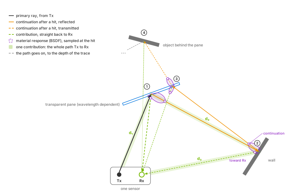— A propagation path from transmitter Tx through a pane, wall and pane to an object behind the glass. Each hit generates one reflected or transmitted continuation and a contribution toward receiver Rx. The highlighted Tx → pane → wall → Rx path has length d₁ + d₂ + d₃, which determines its arrival time. The contribution from behind the pane crosses it again on the return path.#

At each hit, the bidirectional scattering distribution function (BSDF) is evaluated for the continuation and receiver directions. Surface interactions reduce the remaining energy; transmission also depends on wavelength. The diagram shows refraction toward the pane’s normal and traces the path to the configured depth.

Indirect paths can produce ghost detections whose reported range exceeds the geometric distance to either surface.

For a direct-path return, radial velocity is the component of relative motion along the line of sight; purely transverse motion produces no Doppler. Multipath returns also depend on motion projected along the other path segments.

RadialVelocityMs is signed, negative for an approaching detection. Moving or articulated surfaces can produce several velocity contributions when their motion is represented in the scene and the configured velocity resolution can separate them. Seeing scene motion within a step needs the renderer’s motion BVH; refer to Motion BVH.

Simulated effects#

The model simulates the following effects. See mode-specific controls for their attributes.

Phenomenon	What you observe
Field of view and antenna sensitivity	Targets outside the configured angular interval are rejected unless angular aliasing is enabled. Within the interval, the transmit and receive gain patterns change the strength of a return with its direction. Default cosine falloff produces weaker returns toward the edges of the field of view.
Materials and radiometry	Material assignment, incidence geometry, wavelength, antenna gain and distance set the strength and the RCS of a return. Incorrect or missing non-visual material data changes detection. See Non-Visual Sensor Materials and RCS calibration.
Multipath and ghost detections	Indirect propagation paths produce additional detections with shifted range, angle, velocity or RCS. Scene geometry and material response determine their strength. Trace depth limits path length in surface interactions; antenna patterns and detection thresholds also affect which paths produce detections.
Motion and Doppler	Sensor and target motion change radial velocity, and several moving surfaces create a velocity spread when the motion and the geometry are represented and resolvable. See motion BVH and Simulate Moving Targets.
Range, angle and velocity ambiguity	Values outside an unambiguous interval are discarded or folded into that interval, producing an aliased range, angle or radial velocity. Each frame reports its scan’s unambiguous limits; see Outputs.
Detection and false alarms	Weak arrivals are removed, while configured noise varies the measured values or changes which arrivals cross the threshold.
Fidelity and performance	Denser geometric sampling, more propagation depth and larger datacubes resolve more arrivals but need more processing and memory.

Motion BVH#

Radial velocity from scene motion requires an active motion BVH. Select AUTO or ENABLE when creating the renderer; see Motion BVH. Moving-target verification covers the output without motion BVH and how to check whether it is active.

Outputs#

Each PointCloud frame contains detections and metadata identifying the scan configuration and its unambiguous range, velocity and angle limits. Use this metadata to identify the scan that produced a frame. Raw signal samples, datacubes and other intermediate processing data are not available as outputs.

Antenna and scan configuration#

Transmit and receive gain patterns are independent. They support cosine falloff (default), custom gain grids and steerable patch arrays. See antenna attributes and gain grids. WAVEFORM mode also supports MIMO (multiple input, multiple output) with real or virtual receiving apertures.

A sensor can cycle through multiple scan configurations, each with its own field of view, bins and processing settings; see Run More Than One Scan Pattern. All scans must use the same datacubeMode. WAVEFORM includes sampling and finite-duration transform effects, with different processing costs from FAST. See Choose Parameter Values, transmit power and wavelength.

Applications#

Use this model to generate detection lists for tracking, sensor fusion and obstacle sensing. Automotive radar profiles can combine near and far scans, MIMO arrays and Doppler measurements; the default 3.9 mm wavelength is close to 77 GHz. Robotics profiles can model short-range sensing with material response and multipath effects.

Validate a profile in controlled scenes before using it in larger scenarios; see Validate a Parameterization. Radar, lidar and camera sensors can use the same scene and simulation clock.

Sensor definition#

Apply OmniSensorGenericRadarWpmDmatAPI to an OmniRadar prim and target it from a RenderProduct with a PointCloud RenderVar. Select the detection channels to read. See Sensor Configuration for sensor authoring, Output Configuration for output setup and Sensor Outputs for reading tensors. USD Attributes defines the radar controls. The stepping and mapping workflow is also shown in Your First Lidar Sensor.

The Python and C examples use a moving steel cube and a stationary concrete cube. The approaching steel cube produces negative radial velocities. Python displays detections in Rerun; C prints them. Both examples include an alternative scene with thin steel panels, shown above. See Simulate Moving Targets for the scene and stepping loop, and Outputs for reading detections.

The example’s sensor definition applies the schema and sets output coordinates, a 10 Hz frame rate and the transform:

USDA

#usda 1.0
    def OmniRadar "Radar" (
        prepend apiSchemas = ["OmniSensorGenericRadarWpmDmatAPI"]
    )
    {
        token omni:sensor:WpmDmat:elementsCoordsType = "CARTESIAN"
        double2 omni:sensor:frameRate = (10, 1)

        double3 xformOp:translate = (0, 0, 1)
        float3 xformOp:rotateXYZ = (90, 0, -90)
        uniform token[] xformOpOrder = ["xformOp:translate", "xformOp:rotateXYZ"]
    }

USD Python

from pxr import Gf, Sdf

world = stage.DefinePrim("/World", "Xform")

radar = stage.DefinePrim("/World/Radar", "OmniRadar")
radar.AddAppliedSchema("OmniSensorGenericRadarWpmDmatAPI")
radar.CreateAttribute(
    "omni:sensor:WpmDmat:elementsCoordsType", Sdf.ValueTypeNames.Token, custom=False
).Set("CARTESIAN")
radar.CreateAttribute("omni:sensor:frameRate", Sdf.ValueTypeNames.Double2, custom=False).Set(
    Gf.Vec2d(10.0, 1.0)
)
radar.CreateAttribute("xformOp:translate", Sdf.ValueTypeNames.Double3, custom=False).Set(
    Gf.Vec3d(0.0, 0.0, 1.0)
)
radar.CreateAttribute("xformOp:rotateXYZ", Sdf.ValueTypeNames.Float3, custom=False).Set(
    Gf.Vec3f(90.0, 0.0, -90.0)
)
radar.CreateAttribute(
    "xformOpOrder",
    Sdf.ValueTypeNames.TokenArray,
    custom=False,
    variability=Sdf.VariabilityUniform,
).Set(["xformOp:translate", "xformOp:rotateXYZ"])

Configuration and outputs#

Use USD Attributes for controls and How-To to build and validate a device profile. Read Outputs for detection channels, scan metadata, valid-entry handling and visualization.

For shared behavior, see Runtime Parameter Updates and Non-Visual Sensor Materials. The lidar output-shaping guide explains the coordinate and reference-frame choices also used by radar.