Lidar generic core model

The Lidar generic core model simulates rotary and solid-state scanning lidars. An OmniLidar prim with OmniSensorGenericLidarCoreAPI defines the firing schedule, geometric rays and return processing. Configure its omni:sensor:Core:* attributes to match a device’s specifications and calibration data. For pulse propagation and detector modeling, use the separate Lidar generic wpm model.

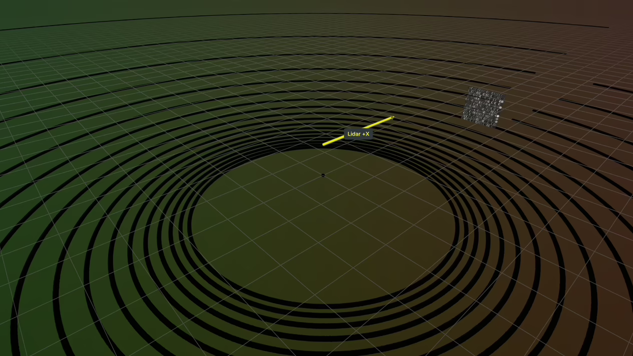
Rotary scan using the default 128-emitter profile. The sensor is 1 m above asphalt, facing a concrete cube 10 m away. Points are shaded by intensity: asphalt is dark and concrete is bright. The arrow marks the forward axis.

Simulation

The model supports rotary and solid-state scans, including flash lidar. Rotary scans repeat a firing pattern through a full revolution, clockwise or counterclockwise, and accept returns within the configured azimuth window. Solid-state scans fire a fixed pattern, arranged in lines, once per scan. omni:sensor:Core:scanType selects the scan type; USD Attributes lists the controls that apply to each.

Each emitter has a firing delay relative to the start of its tick. Points in a scan can therefore have different measurement times, reported by TimeOffsetNs. See Configure a Firing Pattern for scan timing and emitter configuration, USD Attributes for definitions of ticks and emitter states, and Constrain the Field of View for range and azimuth limits.

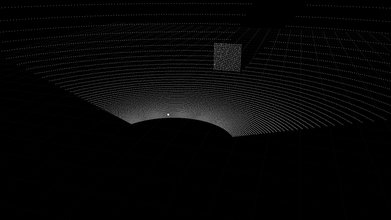
The same scene with ``scanType = SOLID_STATE``: 14,701 emitters in 61 lines at half-degree spacing cover 120 by 30 degrees, firing once per scan. The viewpoint and intensity shading match the rotary scan above.

The default IDEALIZED ray type has no width. GAUSSIAN_BEAM and UNIFORM_BEAM model a finite beam width, with power distributed according to a Gaussian profile or uniformly across the beam. A beam that overlaps an object’s edge can produce returns from both the object and a surface behind it. Beam tracing costs more than idealized rays. See USD Attributes for omni:sensor:Core:rayType, divergence, waist and beam quality.

One firing can produce zero or more returns, up to maxReturns per detector channel. Rays can continue beyond the first surface. The ray type determines which returns are retained; Outputs defines their EchoId order. Range limits, minimum echo separation and the detection threshold can reject returns. Configure these in Constrain the Field of View and Tune Intensity and Point Drops.

Return intensity depends on emitter power, wavelength and pulse duration; detector aperture, efficiency and gain; range; and the surface’s non-visual material. Intensity processing and scaling convert this response to the device’s reflectivity units. The detection threshold is specified by a minimum reflectance and the range at which it must be detected. See Tune Intensity and Point Drops for configuration.

Range accuracy controls distance-dependent measurement noise. Pointing and origin noise perturb each emitter’s direction and beam origin. The means and standard deviations are defined on USD Attributes.

Sensor or target motion during a scan can distort the point cloud. This requires the renderer’s motion BVH. By default, the output retains the distortion; omni:sensor:Core:outputMotionCompensationState enables motion compensation. See Motion Artifacts for both settings and Output Configuration for motion BVH configuration.

Outputs

Each PointCloud RenderVar delivers a composite output of named tensors. Request the channels you need:

• Position: Coordinates, Cartesian or spherical, in sensor, world or custom coordinates.

• Strength and firing time: Intensity and TimeOffsetNs.

• Source of each return: EmitterId, ChannelId, TickId, EchoId and TickState.

• Surface normal and hit-point velocity relative to the sensor: HitNormal and Velocity.

• Material and object identity: MaterialId and ObjectId. Object IDs require a RenderProduct in the scene to request a stable-ID output.

Counts and Flags are always included. Counts bounds the per-return tensors; Flags identifies valid entries.

By default, a complete scan arrives on the step that finishes it. With partialOutputs, each step can deliver the portion of the scan it covers. instantLidar traces a whole scan each step; partialOutputs still controls which steps deliver it. See Outputs for channel definitions and delivery rules, and Sensor Outputs for the container.

Applications

Use this model for geometric point clouds from vehicle-mounted rotary lidars, solid-state robot sensors and industrial single-beam scanners. Build a Profile from a Spec Sheet explains how to create a device profile from a datasheet. The tutorials provide profiles for the Velodyne Alpha Prime (rotary), Blickfeld Cube 1 (solid-state) and SICK TiM781 (both representations).

Multiple sensors can run with one RenderProduct per sensor. Most attributes can be changed while a sensor runs; see Runtime Parameter Updates. Use the Lidar generic wpm model when you need waveform processing, detector response or multipath propagation.

Sensor definition

Apply OmniSensorGenericLidarCoreAPI to an OmniLidar prim. Its defaults define a 128-emitter rotary lidar with one emitter state. Override omni:sensor:Core:* attributes to configure the sensor. Apply additional emitter-state schema instances to alternate between firing patterns.

A RenderProduct targets the sensor through rel camera. Its PointCloud RenderVar selects output channels. Your First Lidar Sensor shows how to create these objects, step the sensor and read valid returns. For reference, see USD Attributes, Sensor Configuration and Output Configuration.

This example applies the schema and sets the output coordinate system, frame rate and sensor transform:

USDA

#usda 1.0
    def OmniLidar "Lidar" (
        prepend apiSchemas = ["OmniSensorGenericLidarCoreAPI"]
    )
    {
        token omni:sensor:Core:elementsCoordsType = "CARTESIAN"
        bool omni:sensor:Core:includeInvalidPoints = false
        double2 omni:sensor:frameRate = (10, 1)

        double3 xformOp:translate = (0, 0, 1)
        float3 xformOp:rotateXYZ = (90, 0, -90)
        uniform token[] xformOpOrder = ["xformOp:translate", "xformOp:rotateXYZ"]
    }

USD Python

from pxr import Gf, Sdf

world = stage.DefinePrim("/World", "Xform")

lidar = stage.DefinePrim("/World/Lidar", "OmniLidar")
lidar.AddAppliedSchema("OmniSensorGenericLidarCoreAPI")
lidar.CreateAttribute(
    "omni:sensor:Core:elementsCoordsType", Sdf.ValueTypeNames.Token, custom=False
).Set("CARTESIAN")
lidar.CreateAttribute(
    "omni:sensor:Core:includeInvalidPoints", Sdf.ValueTypeNames.Bool, custom=False
).Set(False)
lidar.CreateAttribute("omni:sensor:frameRate", Sdf.ValueTypeNames.Double2, custom=False).Set(
    Gf.Vec2d(10.0, 1.0)
)
lidar.CreateAttribute("xformOp:translate", Sdf.ValueTypeNames.Double3, custom=False).Set(
    Gf.Vec3d(0.0, 0.0, 1.0)
)
lidar.CreateAttribute("xformOp:rotateXYZ", Sdf.ValueTypeNames.Float3, custom=False).Set(
    Gf.Vec3f(90.0, 0.0, -90.0)
)
lidar.CreateAttribute(
    "xformOpOrder",
    Sdf.ValueTypeNames.TokenArray,
    custom=False,
    variability=Sdf.VariabilityUniform,
).Set(["xformOp:translate", "xformOp:rotateXYZ"])

The Python and C examples scan a concrete cube above an asphalt plane. They enable motion BVH, warm up the sensor and read a scan using Counts. Both report the valid-point count, mean intensity and largest time offset; the Python example also displays the point cloud in Rerun, as shown above.

Configuration and outputs

Use USD Attributes for controls, How-To for configuration tasks, and Outputs for channel layouts and valid-point handling. The tutorials turn three device datasheets into profiles.

• USD Attributes
• How-To
• Outputs
• Tutorials

Related

• Your First Lidar Sensor — sensor setup, rendering and output mapping.

• Sensor Configuration — instantiating a sensor prim, applying its schema and overriding attributes.

• Output Configuration — RenderProducts, RenderVars and renderer settings, including motion BVH.