Tutorials

These tutorials derive Lidar generic core model profiles from manufacturer specifications. Each includes a completed USD layer you can reference into a scene, the source of each parameter and checks against the device’s published behavior. See Lidar generic core model for model capabilities and How-To for individual configuration tasks.

See Build a Profile from a Spec Sheet for the profiling method.

Tutorial profiles

Parameterize a Rotary Lidar: Velodyne Alpha Prime derives a 128-channel rotary profile from the manual’s nominal channel angles and firing sequence, including maintenance gaps. It relates RPM, frame rate and rotPatternFiringResDeg so changes preserve the firing rate. The resulting layer is Velodyne_Alpha_Prime_Rev4.usda.

Parameterize a Solid-State Lidar: Blickfeld Cube 1 derives a solid-state MEMS pattern from the manufacturer’s mirror equations. It calculates 5,850 directions and firing times and documents four conflicts in the published specifications. It includes Blickfeld_Cube1_Analytic.usda and generate_blickfeld_cube1_profile.py for regenerating the pattern.

Parameterize One Sensor Two Ways: SICK TiM781 models a single laser and detector scanning 811 directions over 270 degrees at 15 Hz. SICK_TiM781.usda uses a rotary emitter; SICK_TiM781_SolidState.usda uses 811 explicit directions and firing times. The rotary schedule scales with scan rate. The solid-state timing must be regenerated when the rate changes.

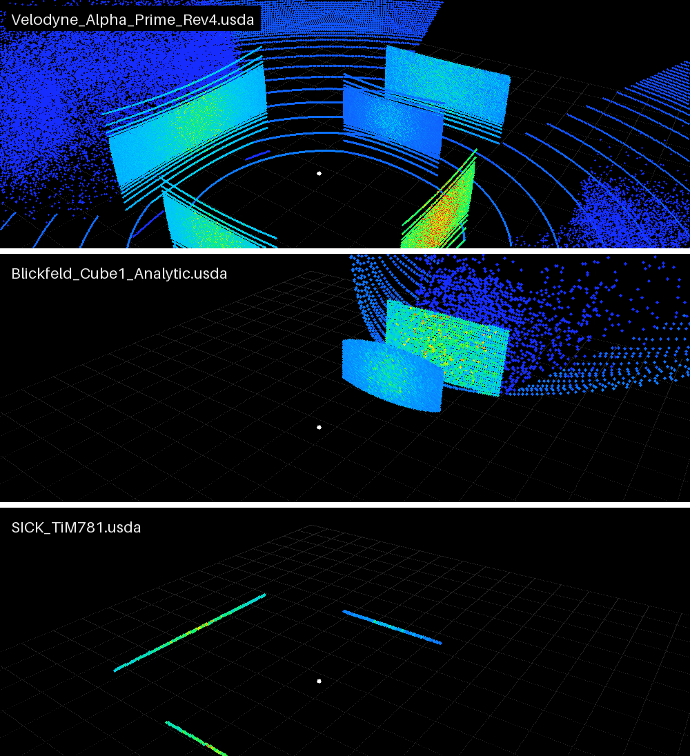
The three shipped profiles referenced into the panel scene at one mount, one below the other, each scan shaded by Intensity: the Alpha Prime’s 128-line rotary sweep, the Cube 1’s Lissajous frame of 5,850 pulses on the pane ahead and the wall behind it, and the TiM781’s single 270-degree plane, which meets only the panels at its height. The layers are Velodyne_Alpha_Prime_Rev4.usda, Blickfeld_Cube1_Analytic.usda and SICK_TiM781.usda under tutorials/assets/.

• Parameterize a Rotary Lidar: Velodyne Alpha Prime
• Parameterize a Solid-State Lidar: Blickfeld Cube 1
• Parameterize One Sensor Two Ways: SICK TiM781

Configuration topics

Each tutorial identifies its sources using source-confidence categories, derives a profile, references it into a scene and validates it. Checks cover parameter acceptance, geometry, timing, range, intensity and comparison with real captures. The following pages explain individual configuration tasks:

• Configure a Firing Pattern: the emitter array lengths, the fire-time order, fractional ticks, channel ids and the minimum scan rate.

• Constrain the Field of View: the azimuth window and the range band.

• Tune Intensity and Point Drops: divergence versus waist and point drops.

• Configure Lidar Output: partialOutputs, scan completion and steps that deliver no points.

• Motion Artifacts: the motion BVH and the compensation state and the compensation tokens.

• USD Attributes: attribute namespaces, the scan type, the parameter validation, range accuracy versus resolution and why channel ids are labels.

• Sensor Configuration: model identity.

• Outputs: reading the points back, Counts, the valid entries and the channel layout.

• Sensor Definition Validation: the introspection parameter validation.

• Output Configuration: the RenderProduct and RenderVar each profile layer carries.

Reading order

For rotary sensors, start with Parameterize a Rotary Lidar: Velodyne Alpha Prime. For solid-state patterns, start with Parameterize a Solid-State Lidar: Blickfeld Cube 1, including its treatment of conflicting sources. Parameterize One Sensor Two Ways: SICK TiM781 compares both representations on one device.

Each layer includes an OmniLidar and a RenderProduct requesting PointCloud. The tutorials show how to reference the default prim, select channels, validate the layer before rendering and compare the results with measured data.

Note

The profiles are documentation-derived baselines, not certified digital twins of a particular hardware unit. Each contains what can be copied or reasonably inferred from the public manuals. Behavior those sources do not define, such as unit-specific optical power, receiver response and thresholds, noise, corrections and the intensity transfer, stays generic or approximate and has to be tuned against measured sensor data for higher-fidelity use.

Related

• Lidar generic core model — what the model simulates, its vocabulary and when to choose it.

• USD Attributes — every attribute the tutorials author, with units, defaults and relations.

• How-To — one page per decision the tutorials make along the way.

• Build a Profile from a Spec Sheet — the method the tutorials work end to end.

• Configure a Firing Pattern — emitter arrays, ticks and fire times.

• Constrain the Field of View — the azimuth window and the range band.

• Tune Intensity and Point Drops — beam shape, intensity and when a return is dropped.

• Configure Lidar Output — coordinates, frame of reference and delivery cadence.

• Motion Artifacts — motion effects while the scan is in progress, and their compensation.

• Outputs — the point cloud the profiles deliver and how to read it back.

• Sensor Definition Validation — the introspection utility behind the parameter validation.

• Output Configuration — the RenderProduct and RenderVars a profile layer carries.

• Python: Camera calibration — the other worked procedure in these docs, from photographs to a calibrated camera.